Bruce Gary, Last updated: 2018.08.12 19 UT
This web page has been "retired"
because it already has too many items for downloading,
and any more additions to it would just make it even
slower to download. The last observation date
described on this web page is 2018.08.01.
Later date observations are described at
ts7.
Since I have probably observed KIC846 more than anyone, I may have earned the right to comment about the suggestion of "alien mega-structures" as a possible explanation for the unexplained dimming behavior before natural explanations had been exhausted. I'm going to repeat a complaint by the Dutch astronomer Ignas Snellen of Leiden Observatory, but first I want to present a brief justification for my right to complain by describing my pro-SETI credentials: 1) In the 1950s I demonstrated the feasibility of an alien civilization in our interstellar neighborhood to broadcast its location by transmitting a map of how constellations appeared from their location, and 2) when I led the JPL Radio Astronomy Group in 1968 I suggested that SETI should be a group goal with a Deep Space Station radio telescope, which my successor eventually did, using DSS-14, until it was killed by a Nevada senator who complained about this NASA project. (As an aside, I was hired at JPL in 1964 by Frank Drake who was apparently impressed by my Jupiter observations with the radio telescope he used for Project Ozma). OK, here's what Dr. Snellen wrote (from link): "...there is no place for alien civilizations in a scientific discussion on new astrophysical phenomena, in the same way as there is no place for divine intervention as a possible solution. One may view it as harmless fun, but I see parallels in athletes taking banned substances. It may lead to short-term fame and medals, but in the long run it harms the sport. Same for astronomy: we should be very careful not to be ridiculed. I really hope we can stop mentioning SETI for every unexplained phenomenon.” The article (by Elizabeth Howell) ends with a quote from Morris Jones, an Australian space observer: "The media is under pressure to deliver attention-grabbing news, but it’s hard to expect them to judge fringe SETI as spurious when it comes from reputable institutions and qualified researchers. The best way to reduce these reports is to stop the production of questionable scientific papers in the first place.” Amen!
_____________________________________________________________________________________________________________________________________
Links on this web page
g', r' & i' Magnitude vs. date
V-mag and g'-mag vs. date
Comparison with AAVSO observations
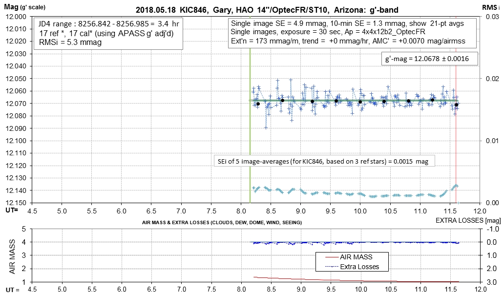
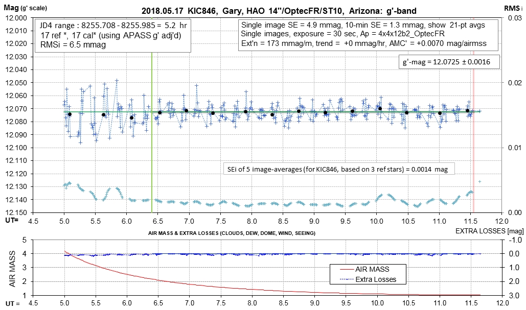
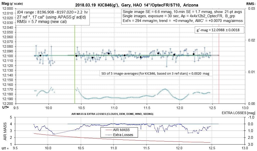
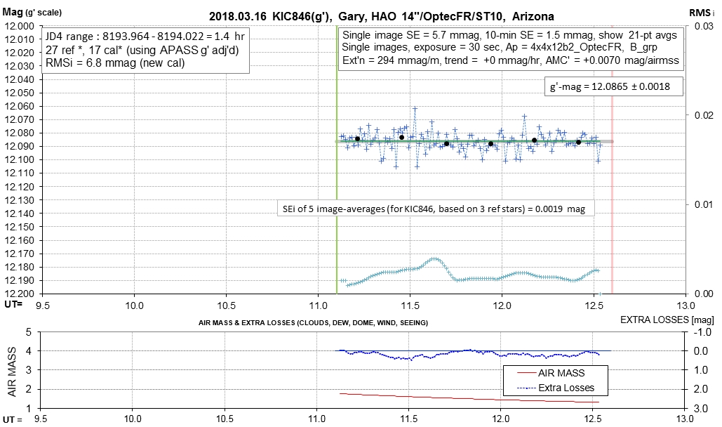
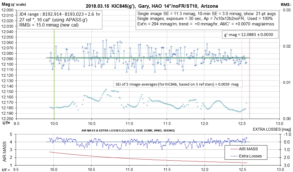
List of observing sessions
Finder image showing new set of reference stars
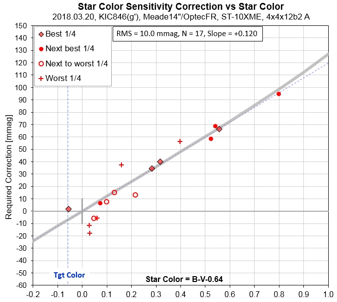
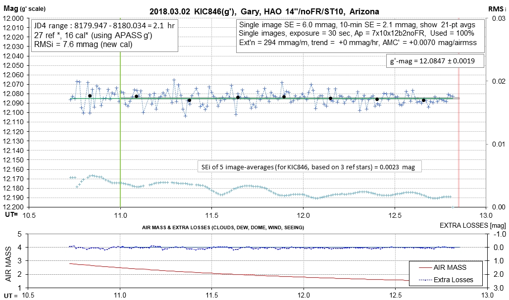
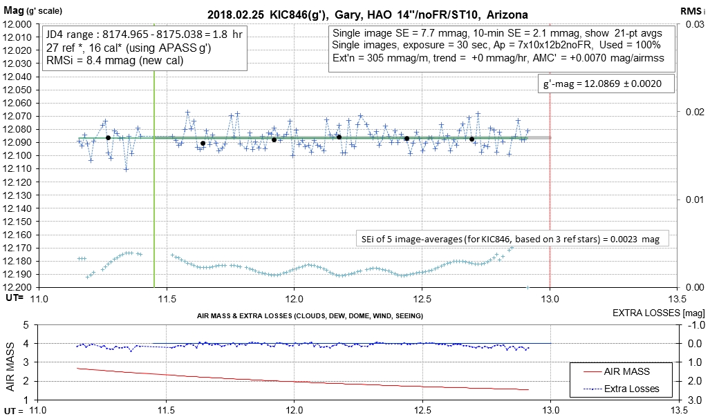
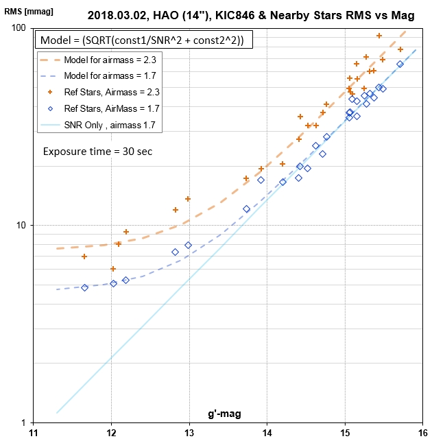
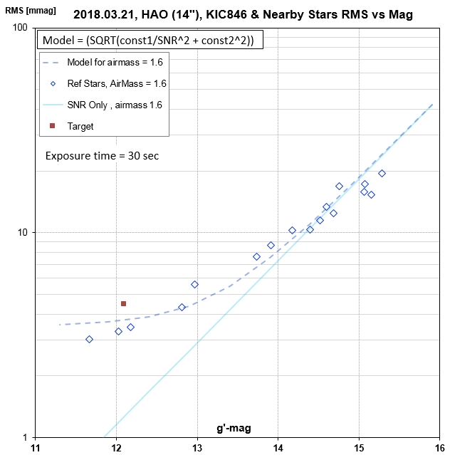
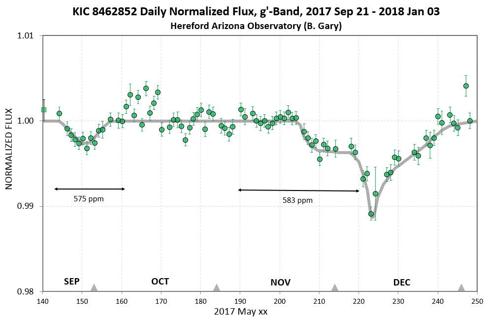
HAO precision explained (580 ppm)
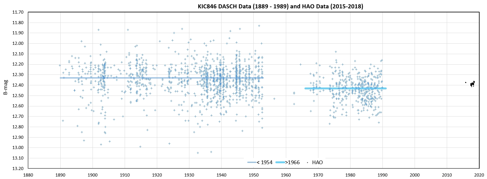
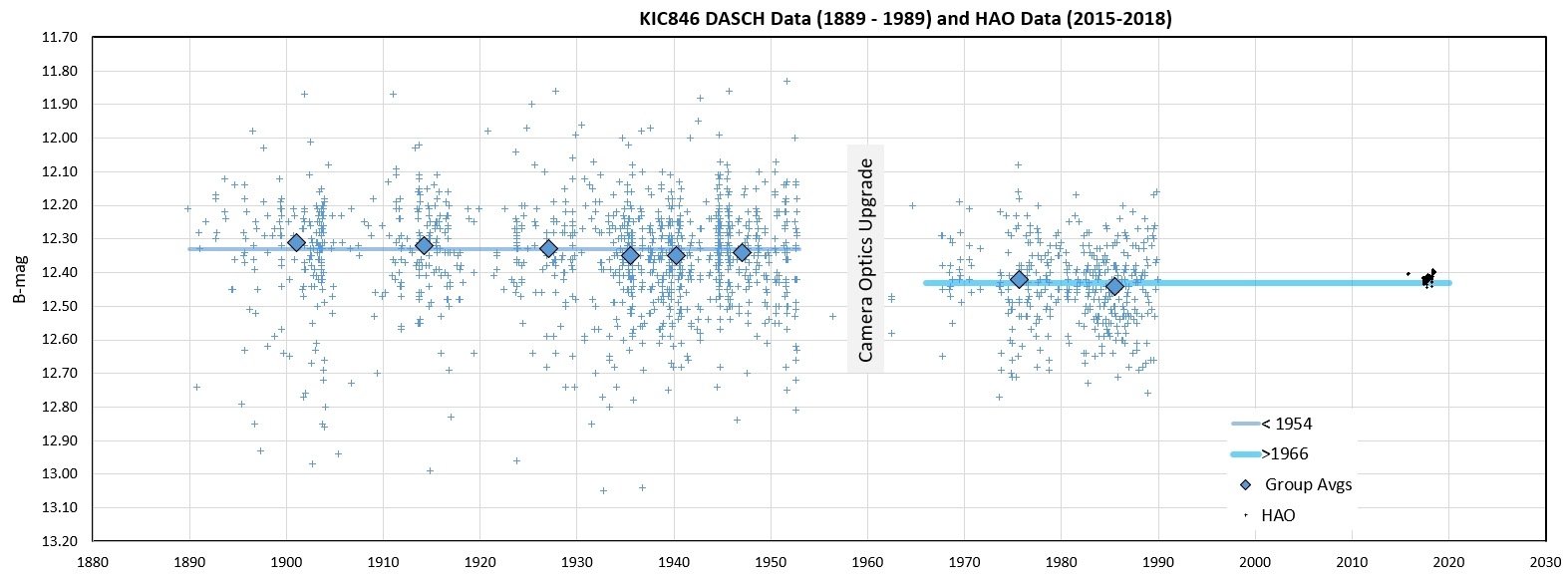
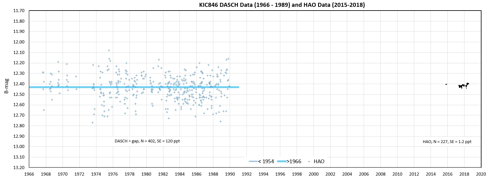
DASCH comment
My collaboration policy
References
Go to 7th of seven web pages.
This is the 6th web page.
Go to 5th of seven web pages (for dates 2017.11.13 to 2018.01.03)
Go to 4th of seven web pages (for dates 2017.09.21 to 2017.11.13)
Go to 3rd of seven web pages (for dates 2017.08.29 to 2017.09.18)
Go to 2nd of seven web pages (for dates 2017.06.18 to 2017.08.28)
Go to 1st of seven web pages (for dates 2014.05.02 to 2017.06.17)
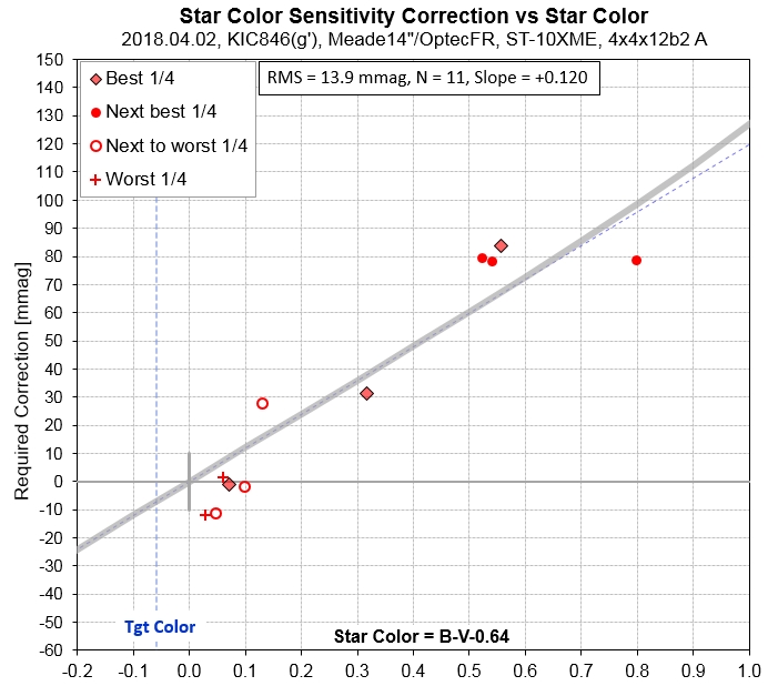
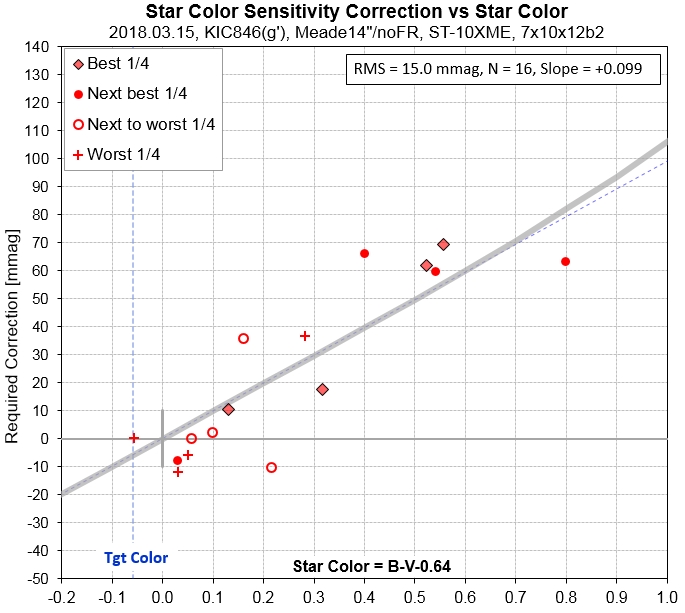
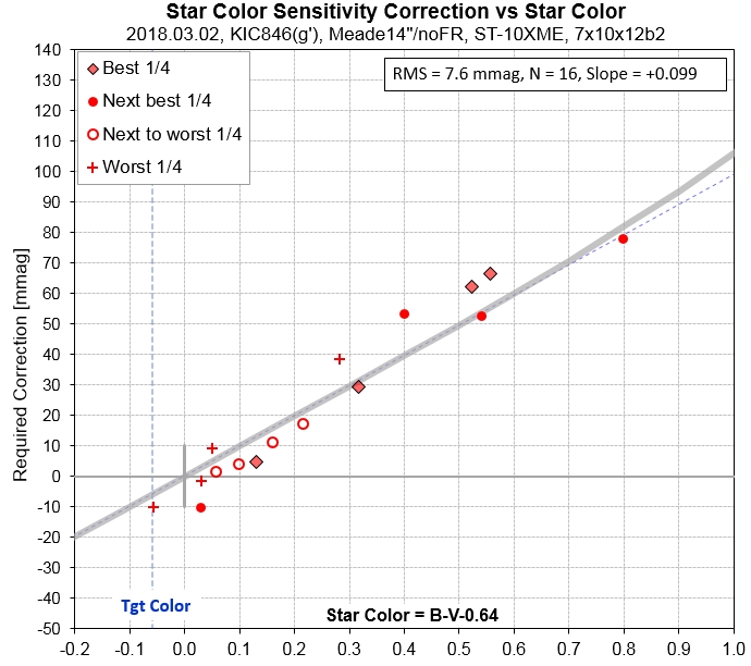
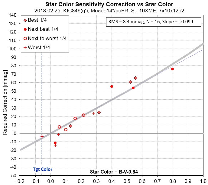
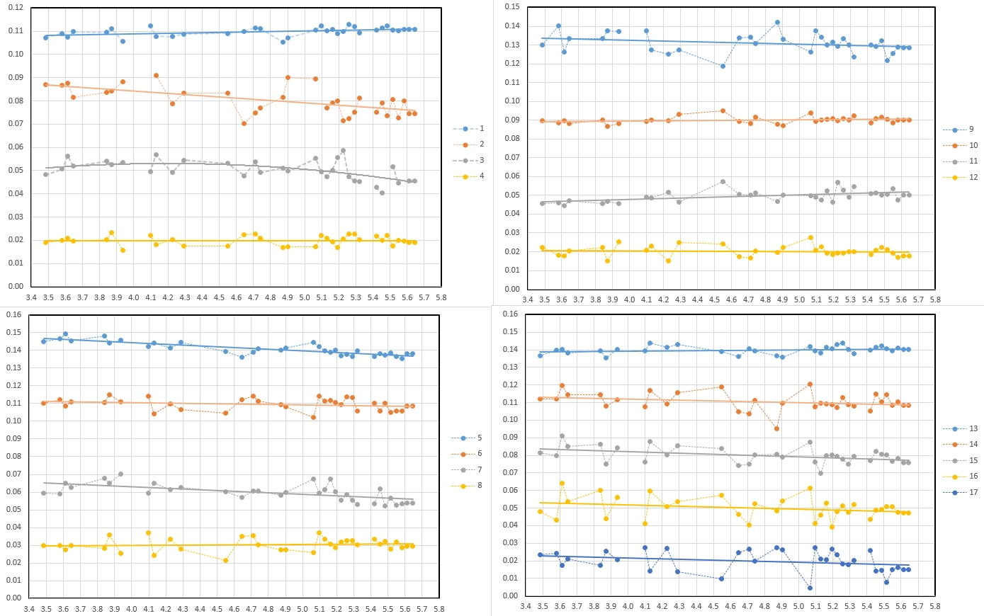
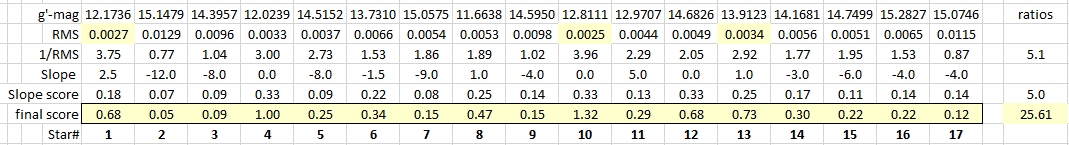
Reference Star Quality Assessment (the 10 best stars out of 25 evaluated)
This is the 6th web pages devoted to my observations of Tabby's Star. When a web page has many images the download times are long, so this is the latest "split."
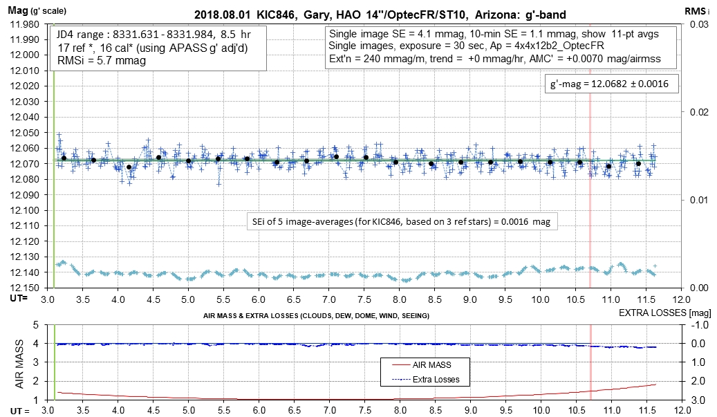
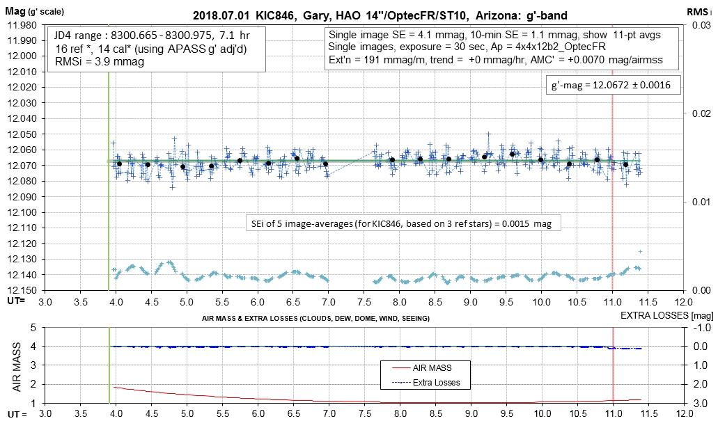
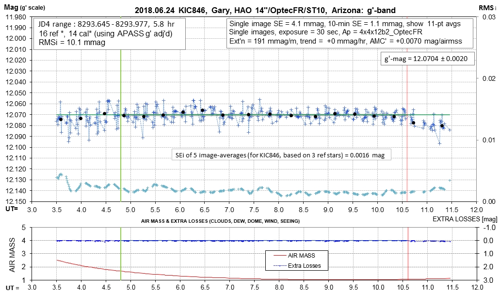
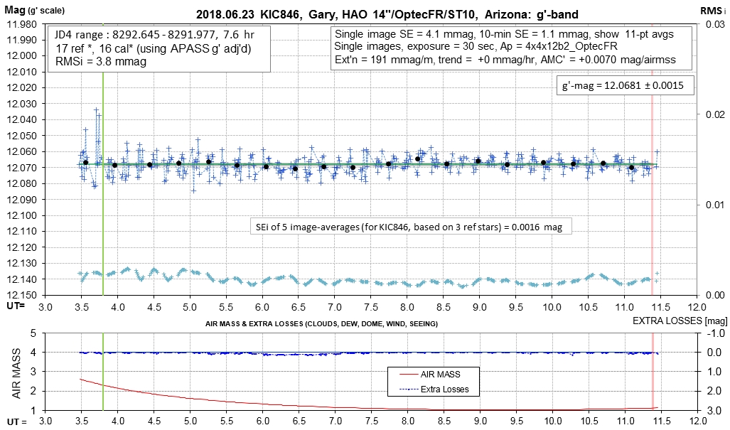
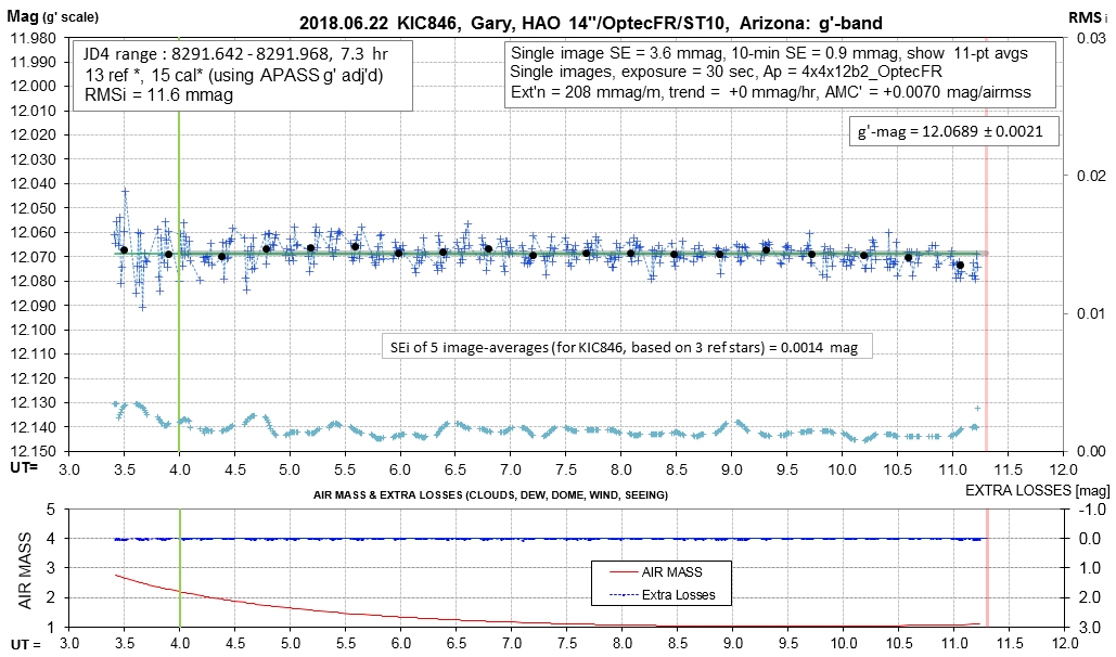
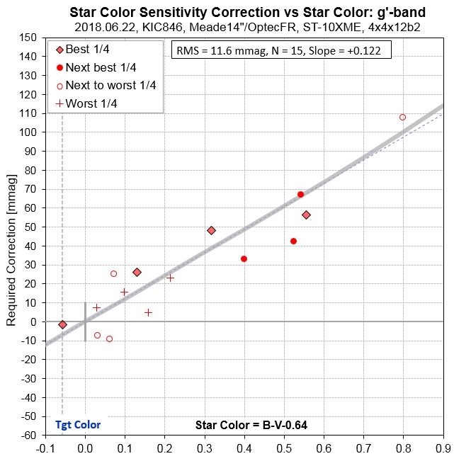
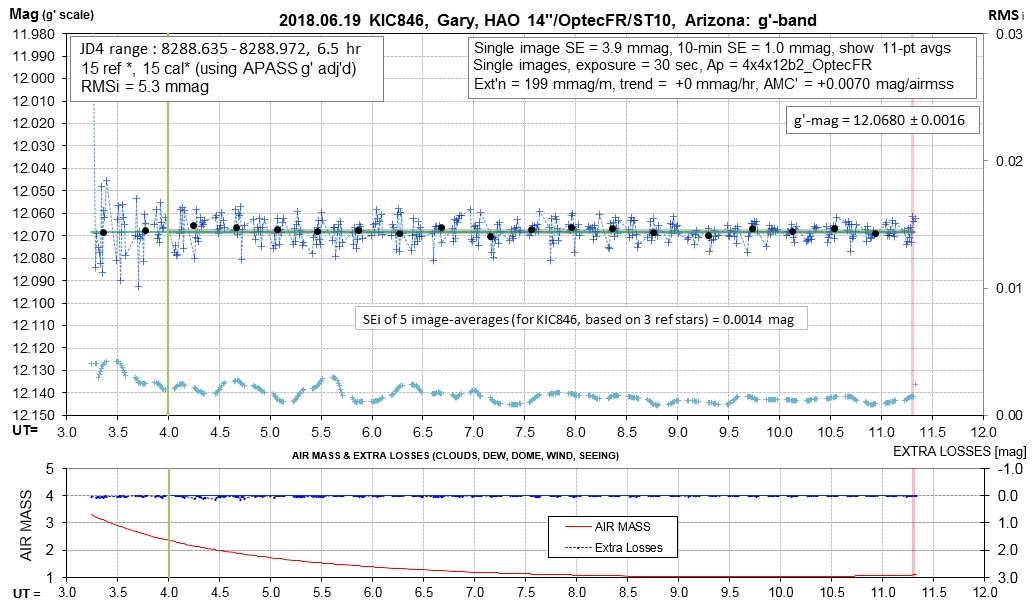
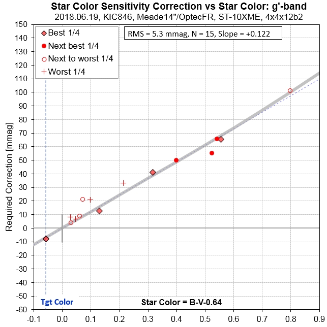
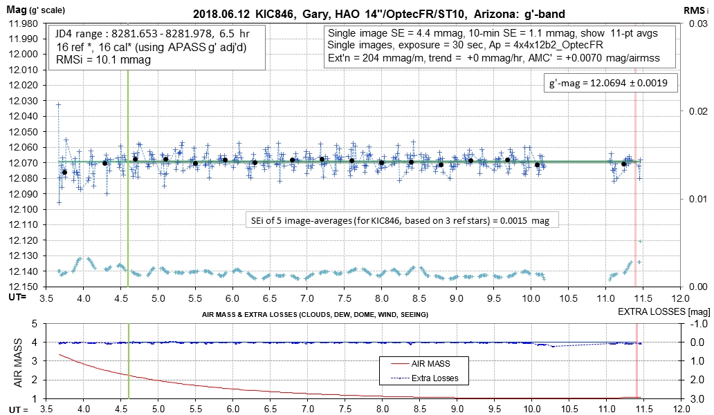
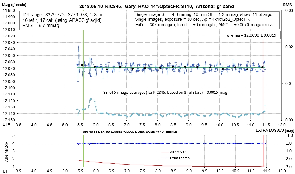
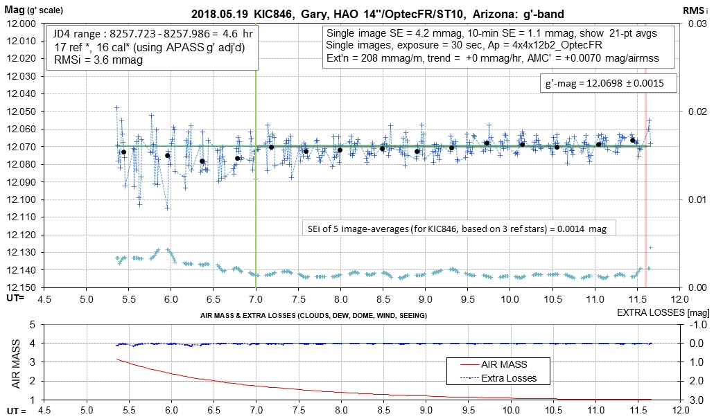
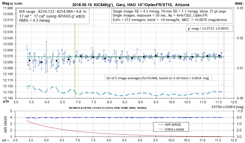
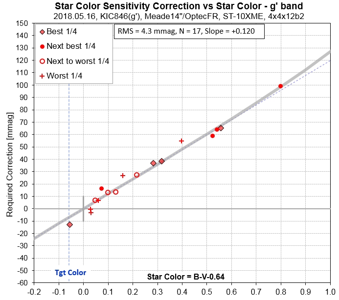
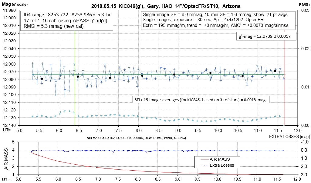
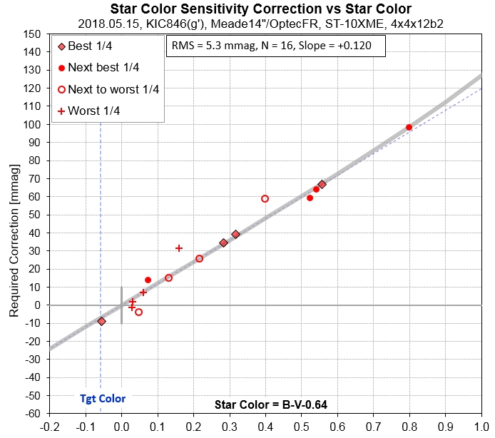
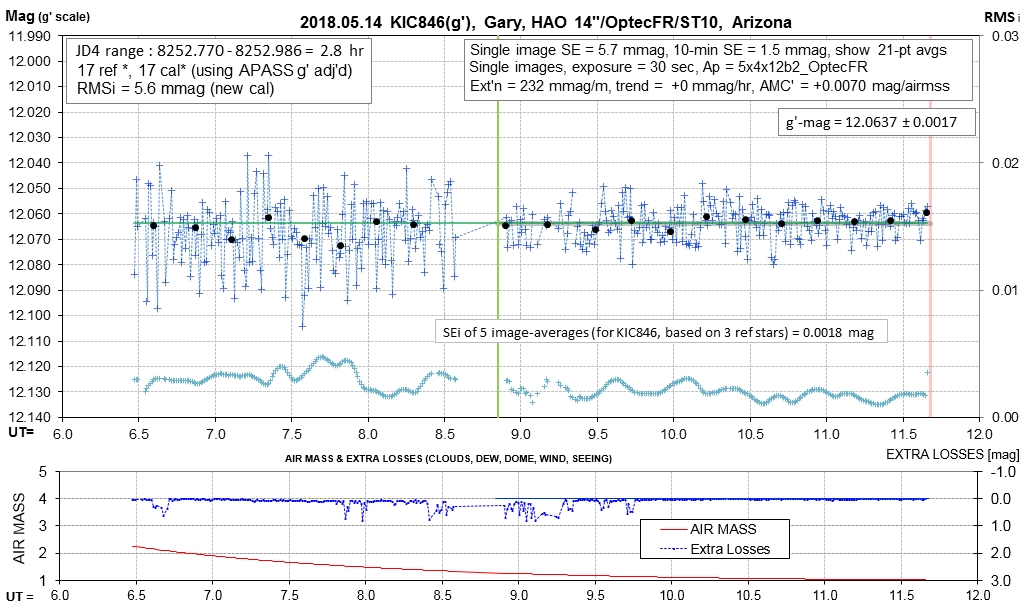
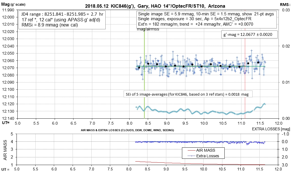
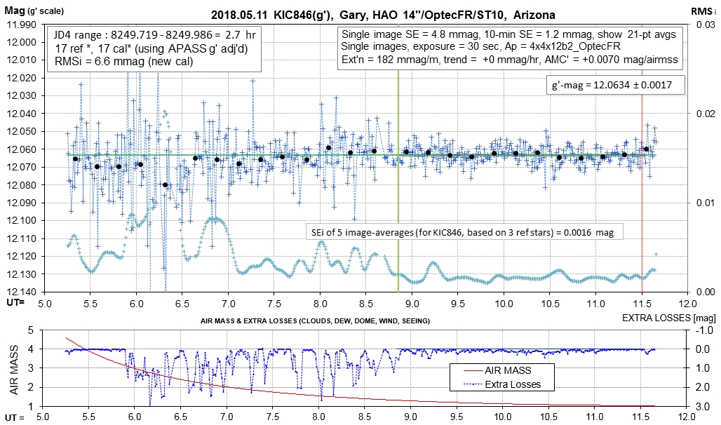
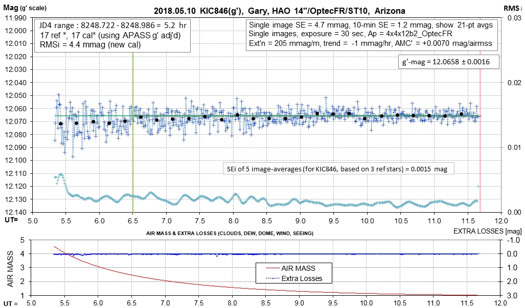
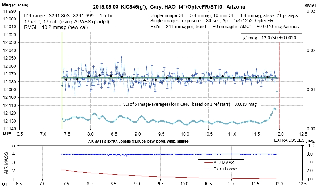
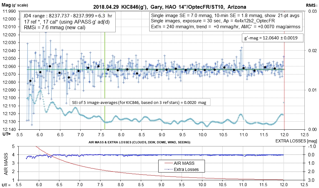
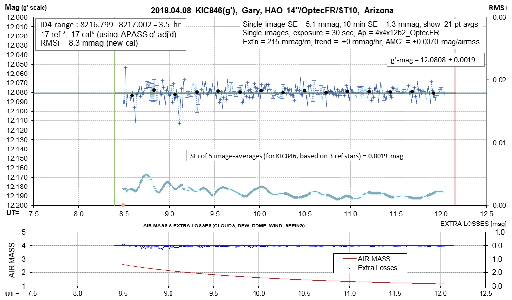
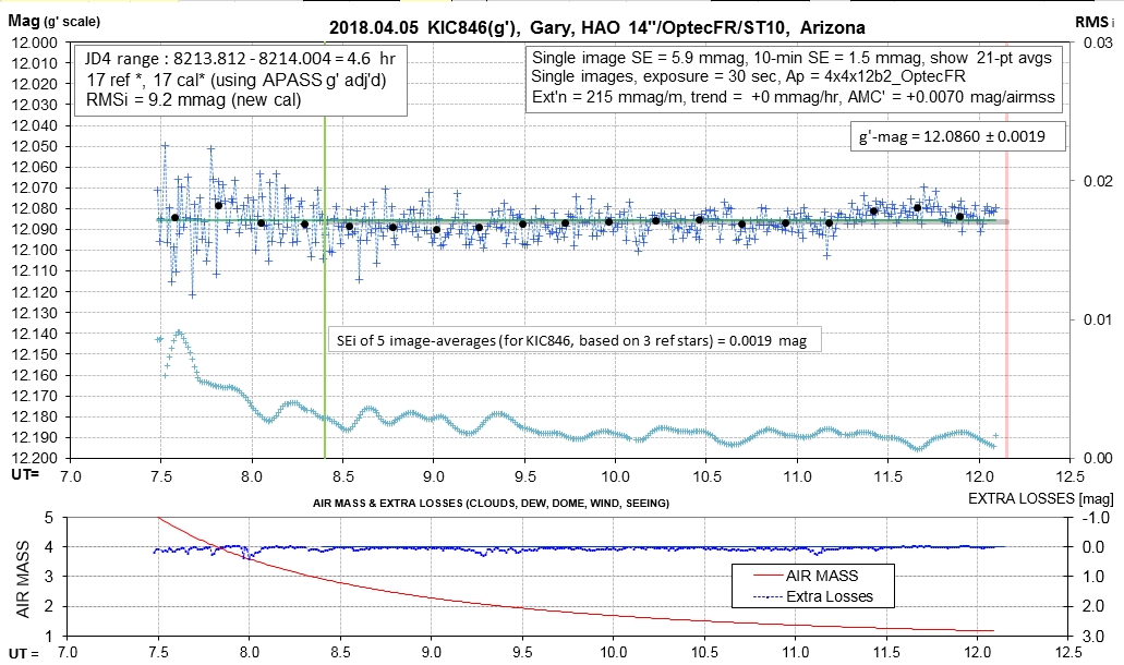
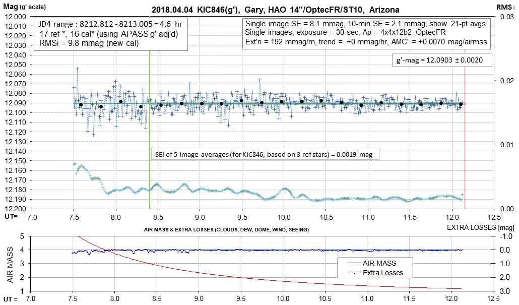
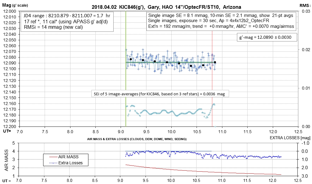
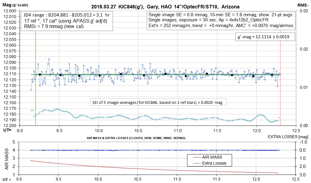
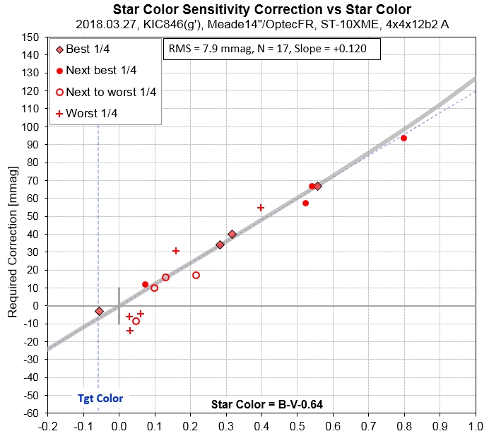
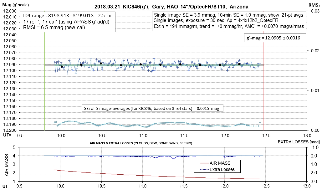
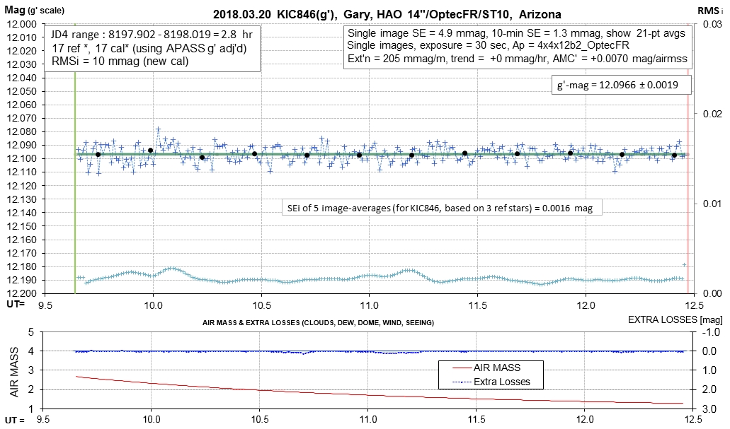
g', r' and i' Mag's vs. Date
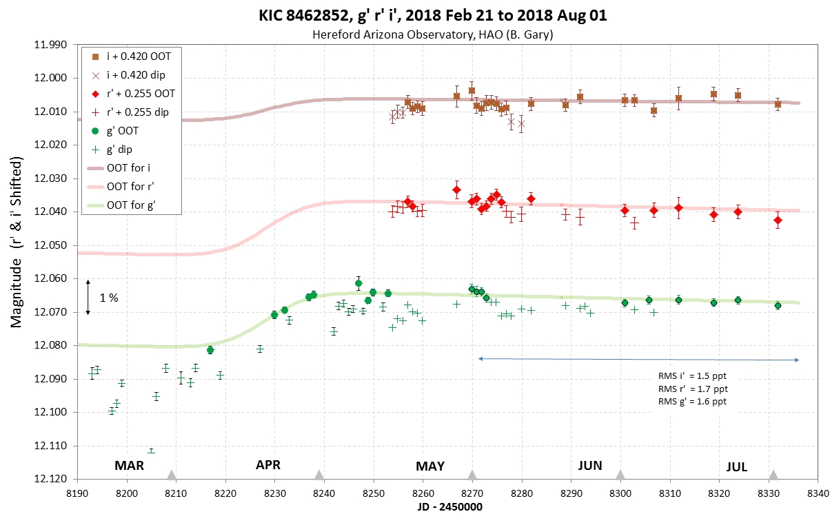
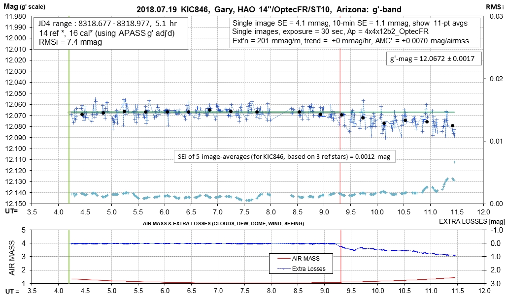
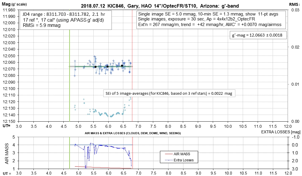
Figure 1. HAO magnitudes at g'-band for the past 2.5 months. The "OOT only" trace is the second "U-Shaped" component needed to account for the upper-boundary of measurements (presumably the out-of-transit, or OOT, level).
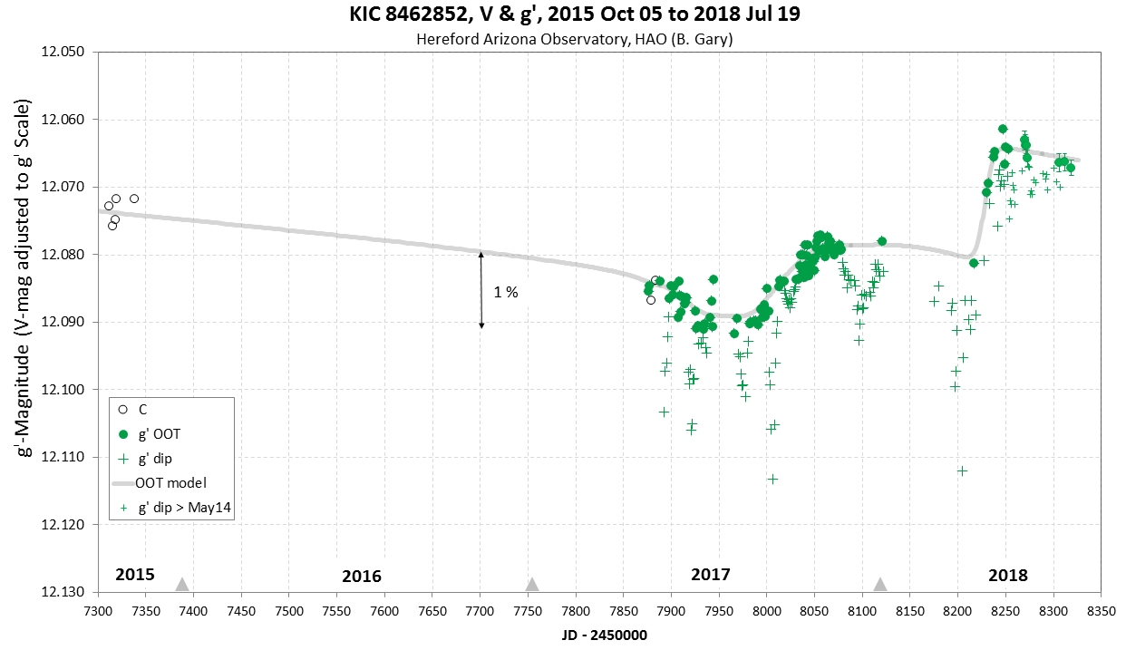
V and g'-Mag vs. Date
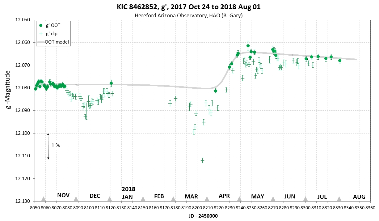
Figure 2. HAO magnitudes at g'-band for the past 7 months. The "OOT only" trace is the second "U-Shaped" component needed to account for the upper-boundary of measurements (presumably the out-of-transit, or OOT, level).
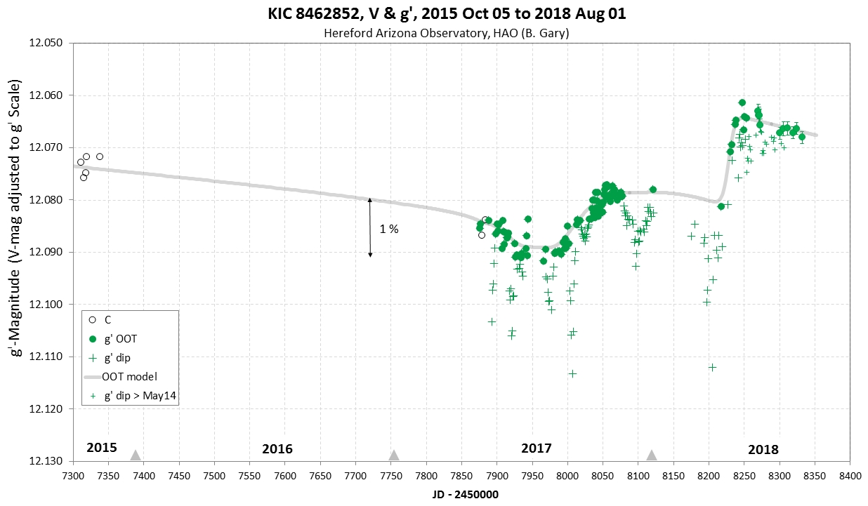
Figure 3. This shows the last 2.5 years of C-, V- and g'-band HAO measurements (C- and V-mag's adjusted to match g'-mag's).
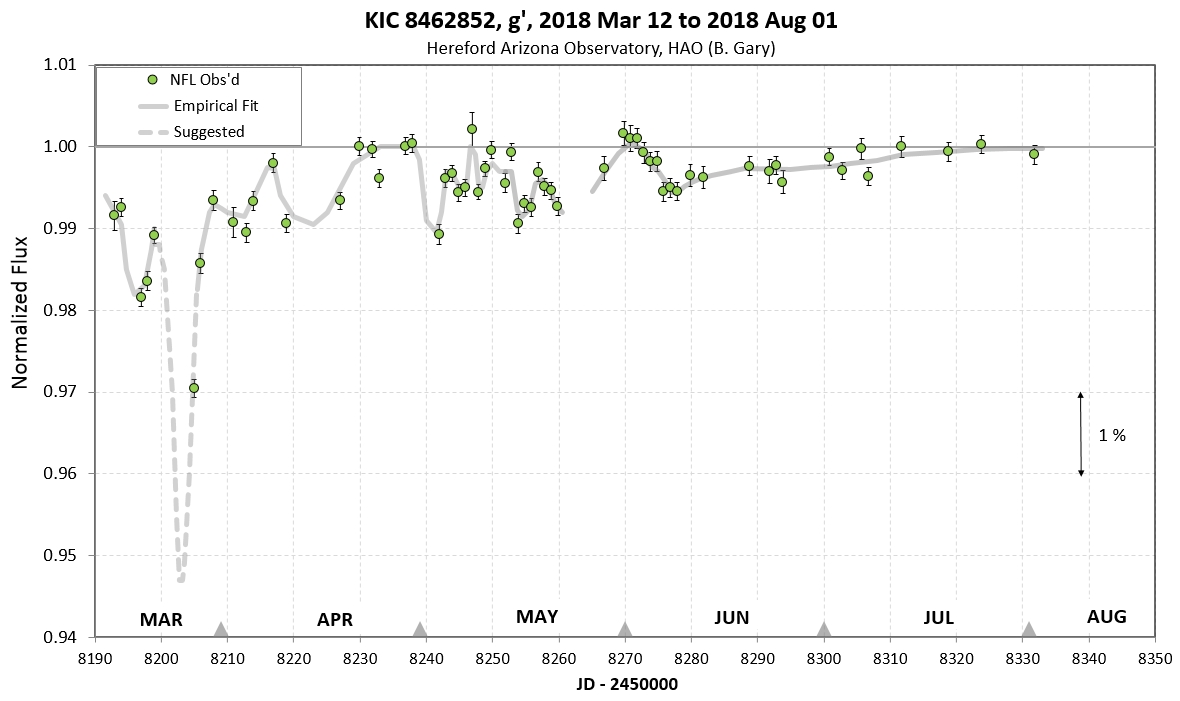
Figure 4. Normalized flux light curve for the past 2 months, based on the OOT model shown in the previous two graphs.
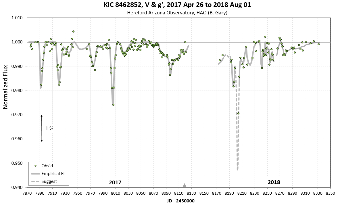
Figure 5. A one-year plot of "normalized flux" based on the previously displayed OOT model (with two U-shaped features). The HAO data for April are too sparse for showing dip structure well; the graphs in the next section do a better job of that sine they include AAVSO measurements.
Comparison of HAO with AAVSO Observations (Demonstration of the value of combining AAVSO data with other data with emphasis on the biggest ground-based observed dip.)
The following figure shows a selection of AAVSO observer V-band magnitudes vs. date for a 2.6-year interval.
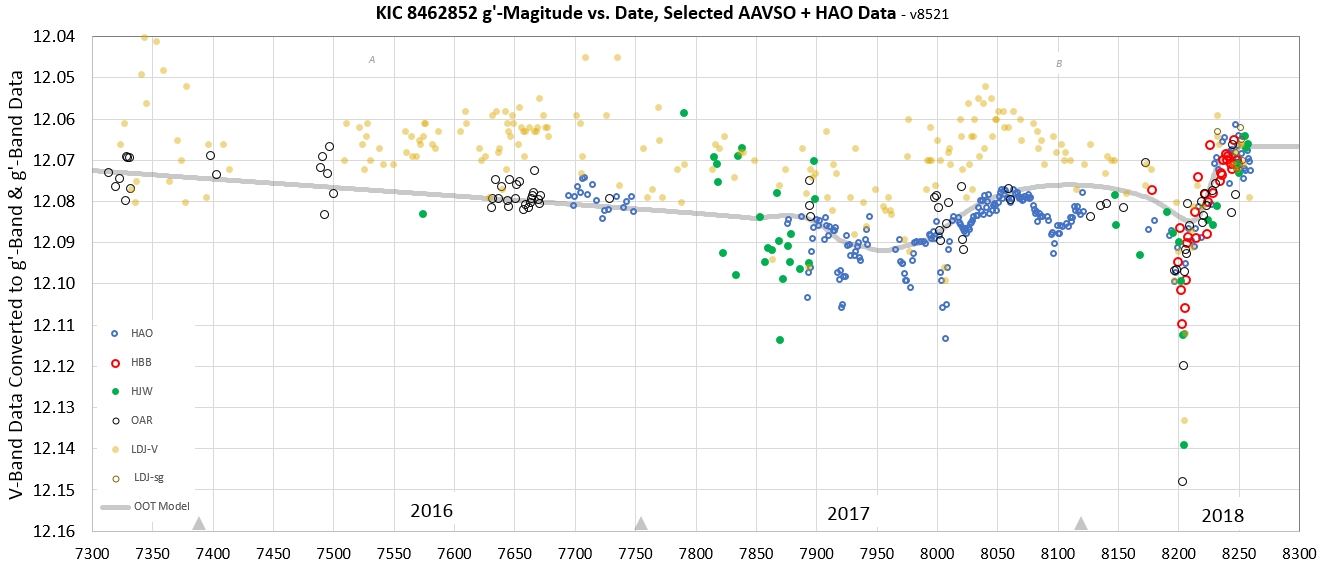
Figure 6a. Selected AAVSO plus HAO V-band (and g'-band) magnitudes for a 2.6-year interval. Offsets for each observer were applied to achieve agreement with HAO data. Two U-shaped features are included in the OOT Model. Observers: OAR = Arto Oksanen (Finland), HBB = Barbara Harris (Florida, USA), HJW = John Hall (Colorado, USA), LDJ = David Lane (Nova Scotia, Canada).
During the first 2 years a steady fade is present (confirming last year's interpretation of HAO data). It is interrupted by a U-shaped fade feature in mid-2017, and is followed by a second U-shaped fade in early 2018. The "OOT model" trace is meant to show what would be observed if dips did not occur, so it can serve as a reference level for determining dip depth and shape. The deepest dip occurs at ~ JD4 = 8203 and is ~ 67 mmag (~ 6 %) deep.
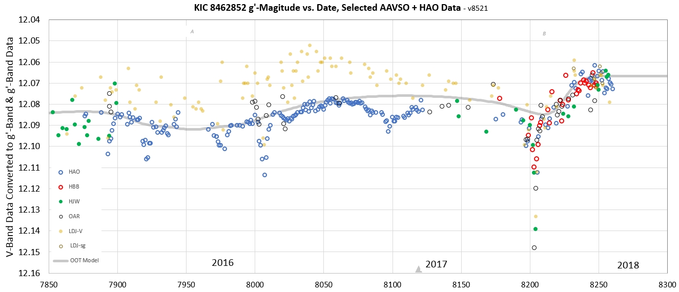
Figure 6b. Same data as above, but showing just the last year of data.
David Lane (AAVSO Observer Code LDJ) has reprocessed his 2.6 year's of KIC846 observations (lot's of work!), and has re-submitted them to the AAVSO database. The LDJ V-band data for times of known dips were excluded, and the remaining OOT (out-of-transit) data was averaged in groups of 7 observing sessions. An arbitrary offset was applied to achieve maximum agreement (this is legitimate since every observer has a unique and unknown absolute calibration uncertainty). The purpose for performing these adjustments was to allow for an assessment of the presence of a U-shaped OOT pattern with an approximate 1-year timescale that has been derived using HAO data. The next figure is a light curve showing how the LDJ V-mag measurements compare with HAO data.
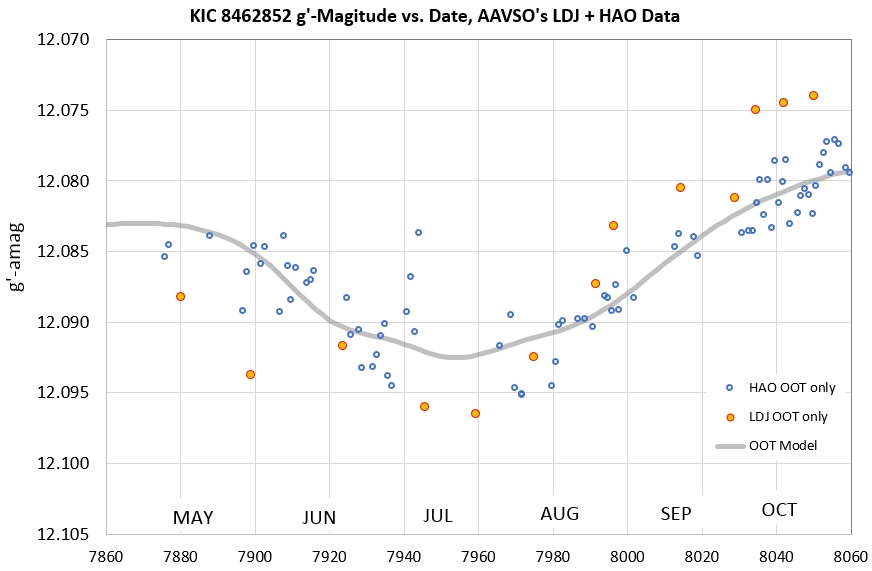
Figure 7. Six-month light curve for two observers, LDJ (David Lane) and HAO (Bruce Gary). The LDJ symbols are averages of 4 observing sessions (~ 25 images per session) while the HAO symbols are for individual observing sessions (>200 images per session, typically). Dip data for both LDJ and HAO have been excluded from this LC. The LDJ and HAO symbols can therefore be viewedd as OOT only. Both data sets confirm the U-shaped OOT model (centered on mid-2017).
This figure shows agreement of both LDJ and HAO data with the main U-shaped OOT Model.
I conclude that the U-shaped OOT model has support from both data sets. The depth of the U-shape is ~ 1.0 % and the duration of the U-shape is ~ 1.0 year. So far, the LDJ and HAO data agree in suggesting that since the time of maximum brightness at the end of the U-shape (near JD4 = 8050) a steep fade has been underway. LDJ B-band measurements will be presented here that show a greater U-shape depth than for V-band! This will provide a significant constraint on modeling the physical mechanism for the U-shape (large dust cloud vs. reflection of starlight by the dip clouds).
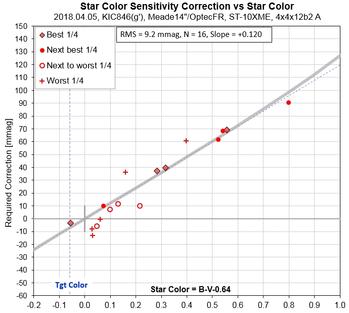
The next graph is a comparison of downloaded AAVSO data for March and April. Data for 5 observers is shown with offsets chosen to maximize agreement with HAO and each other.
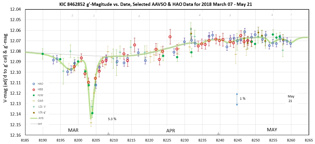
Figure 8. Comparison of g'-mag (and V-mag, adjusted) for 5 AAVSO observers and HAO during March, April and May, 2018. Arbitrary offsets have been applied to each observer data set to achieve agreement with HAO data, where overlap exists, and with each other (i.e., internal consistency). The green trace is the sum of a slowly varying OOT model plus a short-term dip modeled using "asymmetric hyper-secant" (AHS) functions. The 60 mmag dip ( ~ 5.3 %, dip at JD4 = 8203.4) is fitted well by the AHS function. (The data in this figure was downloaded from the AAVSO web site: https://www.aavso.org/lcg.)
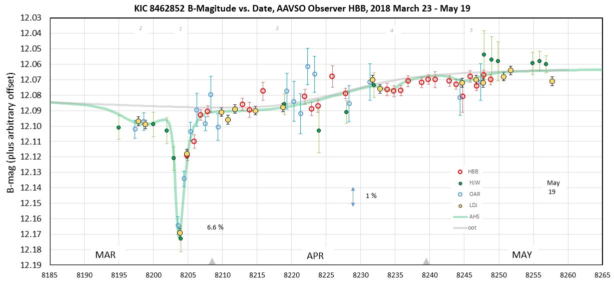
Figure 9. Comparison of B-mag for two AAVSO observers during March, April and May, 2018. Arbitrary offsets have been applied to each observer data set to achieve agreement with HBB data, where overlap exists, and with each other (i.e., internal consistency). The green trace is the sum of a slowly varying OOT model plus a short-term dip modeled using "asymmetric hyper-secant" (AHS) functions. The 82 mmag dip (6.6 %, at JD4 = 8203.4) is fitted well by the AHS function. (The data in this figure was downloaded from the AAVSO web site: https://www.aavso.org/lcg.) [Still working with this graph, adding data from other observers.]
Both V-band and B-band exhibit a significant brightening from early April to early May. There appears to be a small but significant difference in the brightening amount at the two bands. The brightening from 8208 - 8215 to 8237 - 8253 is 13.7 +/- 3.0 mmag at V-band and 20.5 +/- 1.7 mmag at B-band (using a sum of chi squares analysis). The difference in brightening is 6.8 +/- 3.5 mmag, which is significant at the 2.0-sigma level. In other words, there's a 95 % probability that the difference in amount of brightening at B- and V-band is real, with a greater amount of brightening at B-band. If this finding holds up then we would have to invoke a dust cloud model to explain the slow variation (i.e., the U-shaped variations), and that dust cloud would have to include a significant component of small particles (<0.3 micron radius).
The deep dip in late March is also deeper at B-band than V-band. Again, this is evidence for the presence of a significant component of small dust particles in the dust cloud producing this dip.
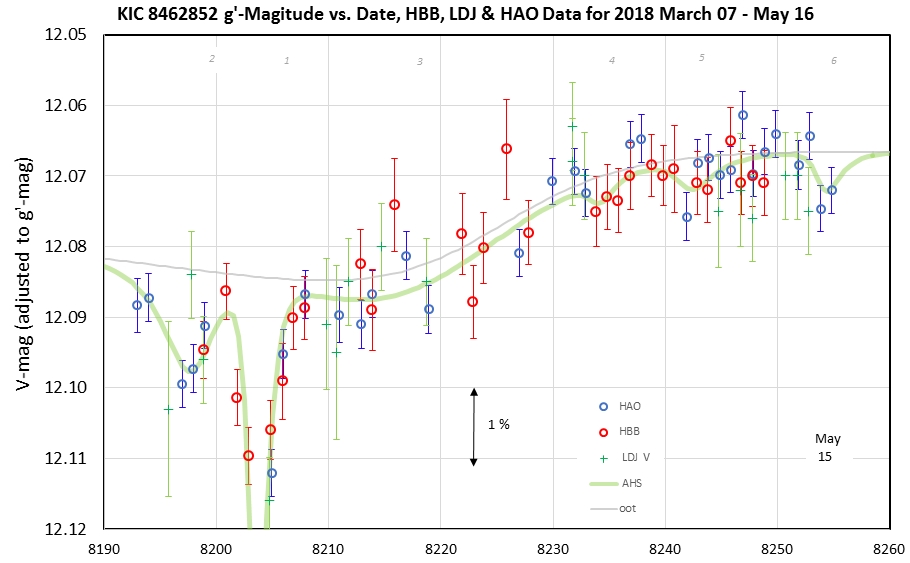
Figure 10. Same as Fig. 7, but showing only HBB, LDJ and HAO data. The good agreement between three independent data sets (showing a dramatic 2 % brightening) suggests that the variations shown are real. A similar graph for B-band shows the same brightening for different observers, again giving credence to the reality of the brightening.
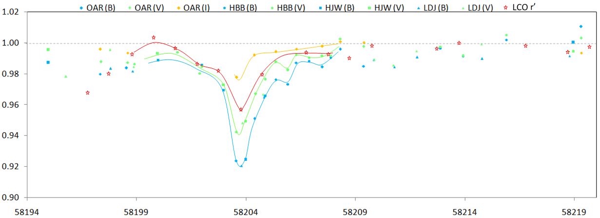
Figure 12. Rafik Bourne's comparison of dip depth for different wavelengths. B-band has the deepest depth while Ic-band has the smallest depth. (The LCO data are manually read off graphs at Tabby's blog, made necessary because these data values are not in the public domain.) Clearly, the dip at JD4 = 8203.5 is due to a dust cloud dominated by a component of small particles (< 0.3 micron radius).
Transit Pattern and Speculation about Model for KIC846 Dust Cloud Geometry (not Physical Mechanism Model)
A thorough description of this matter is given in the 5th web page of this 6-part series of web pages: link.
Since I have probably observed KIC846 more than anyone, I may have earned the right to comment about the suggestion of "alien mega-structures" as a possible explanation for the unexplained dimming behavior before natural explanations had been exhausted. I'm going to repeat a complaint by the Dutch astronomer Ignas Snellen of Leiden Observatory, but first I want to present a brief justification for my right to complain by describing my pro-SETI credentials: 1) In the 1950s I demonstrated the feasibility of an alien civilization in our interstellar neighborhood to broadcast its location by transmitting a map of how constellations appeared from their location, and 2) when I led the JPL Radio Astronomy Group in 1968 I suggested that SETI should be a group goal with a Deep Space Station radio telescope, which my successor eventually did, using DSS-14, until it was killed by a Nevada senator who complained about this NASA project. (As an aside, I was hired at JPL in 1964 by Frank Drake who was apparently impressed by my Jupiter observations with the radio telescope he used for Project Ozma). OK, here's what Dr. Snellen wrote (from link): "...there is no place for alien civilizations in a scientific discussion on new astrophysical phenomena, in the same way as there is no place for divine intervention as a possible solution. One may view it as harmless fun, but I see parallels in athletes taking banned substances. It may lead to short-term fame and medals, but in the long run it harms the sport. Same for astronomy: we should be very careful not to be ridiculed. I really hope we can stop mentioning SETI for every unexplained phenomenon.” The article (by Elizabeth Howell) ends with a quote from Morris Jones, an Australian space observer: "The media is under pressure to deliver attention-grabbing news, but it’s hard to expect them to judge fringe SETI as spurious when it comes from reputable institutions and qualified researchers. The best way to reduce these reports is to stop the production of questionable scientific papers in the first place.” Amen!
_____________________________________________________________________________________________________________________________________
Links on this web page
g', r' & i' Magnitude vs. date
V-mag and g'-mag vs. date
Comparison with AAVSO observations
List of observing sessions
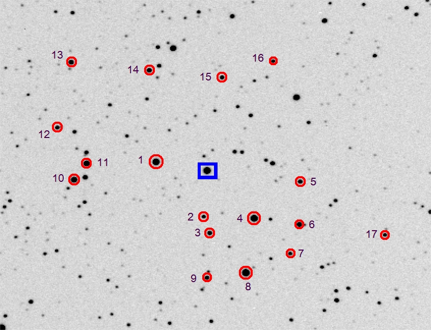
Finder image showing new set of reference stars
HAO precision explained (580 ppm)
DASCH comment
My collaboration policy
References
Go to 7th of seven web pages.
This is the 6th web page.
Go to 5th of seven web pages (for dates 2017.11.13 to 2018.01.03)
Go to 4th of seven web pages (for dates 2017.09.21 to 2017.11.13)
Go to 3rd of seven web pages (for dates 2017.08.29 to 2017.09.18)
Go to 2nd of seven web pages (for dates 2017.06.18 to 2017.08.28)
Go to 1st of seven web pages (for dates 2014.05.02 to 2017.06.17)
Reference Star Quality Assessment (the 10 best stars out of 25 evaluated)
This is the 6th web pages devoted to my observations of Tabby's Star. When a web page has many images the download times are long, so this is the latest "split."
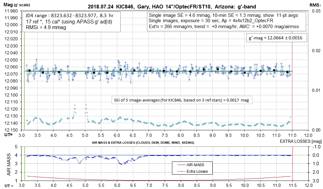
g', r' and i' Mag's vs. Date
Figure 1. HAO magnitudes at g'-band for the past 2.5 months. The "OOT only" trace is the second "U-Shaped" component needed to account for the upper-boundary of measurements (presumably the out-of-transit, or OOT, level).
V and g'-Mag vs. Date
Figure 2. HAO magnitudes at g'-band for the past 7 months. The "OOT only" trace is the second "U-Shaped" component needed to account for the upper-boundary of measurements (presumably the out-of-transit, or OOT, level).
Figure 3. This shows the last 2.5 years of C-, V- and g'-band HAO measurements (C- and V-mag's adjusted to match g'-mag's).
Figure 4. Normalized flux light curve for the past 2 months, based on the OOT model shown in the previous two graphs.
Figure 5. A one-year plot of "normalized flux" based on the previously displayed OOT model (with two U-shaped features). The HAO data for April are too sparse for showing dip structure well; the graphs in the next section do a better job of that sine they include AAVSO measurements.
Comparison of HAO with AAVSO Observations (Demonstration of the value of combining AAVSO data with other data with emphasis on the biggest ground-based observed dip.)
The following figure shows a selection of AAVSO observer V-band magnitudes vs. date for a 2.6-year interval.
Figure 6a. Selected AAVSO plus HAO V-band (and g'-band) magnitudes for a 2.6-year interval. Offsets for each observer were applied to achieve agreement with HAO data. Two U-shaped features are included in the OOT Model. Observers: OAR = Arto Oksanen (Finland), HBB = Barbara Harris (Florida, USA), HJW = John Hall (Colorado, USA), LDJ = David Lane (Nova Scotia, Canada).
During the first 2 years a steady fade is present (confirming last year's interpretation of HAO data). It is interrupted by a U-shaped fade feature in mid-2017, and is followed by a second U-shaped fade in early 2018. The "OOT model" trace is meant to show what would be observed if dips did not occur, so it can serve as a reference level for determining dip depth and shape. The deepest dip occurs at ~ JD4 = 8203 and is ~ 67 mmag (~ 6 %) deep.
Figure 6b. Same data as above, but showing just the last year of data.
David Lane (AAVSO Observer Code LDJ) has reprocessed his 2.6 year's of KIC846 observations (lot's of work!), and has re-submitted them to the AAVSO database. The LDJ V-band data for times of known dips were excluded, and the remaining OOT (out-of-transit) data was averaged in groups of 7 observing sessions. An arbitrary offset was applied to achieve maximum agreement (this is legitimate since every observer has a unique and unknown absolute calibration uncertainty). The purpose for performing these adjustments was to allow for an assessment of the presence of a U-shaped OOT pattern with an approximate 1-year timescale that has been derived using HAO data. The next figure is a light curve showing how the LDJ V-mag measurements compare with HAO data.
Figure 7. Six-month light curve for two observers, LDJ (David Lane) and HAO (Bruce Gary). The LDJ symbols are averages of 4 observing sessions (~ 25 images per session) while the HAO symbols are for individual observing sessions (>200 images per session, typically). Dip data for both LDJ and HAO have been excluded from this LC. The LDJ and HAO symbols can therefore be viewedd as OOT only. Both data sets confirm the U-shaped OOT model (centered on mid-2017).
This figure shows agreement of both LDJ and HAO data with the main U-shaped OOT Model.
I conclude that the U-shaped OOT model has support from both data sets. The depth of the U-shape is ~ 1.0 % and the duration of the U-shape is ~ 1.0 year. So far, the LDJ and HAO data agree in suggesting that since the time of maximum brightness at the end of the U-shape (near JD4 = 8050) a steep fade has been underway. LDJ B-band measurements will be presented here that show a greater U-shape depth than for V-band! This will provide a significant constraint on modeling the physical mechanism for the U-shape (large dust cloud vs. reflection of starlight by the dip clouds).
The next graph is a comparison of downloaded AAVSO data for March and April. Data for 5 observers is shown with offsets chosen to maximize agreement with HAO and each other.
Figure 8. Comparison of g'-mag (and V-mag, adjusted) for 5 AAVSO observers and HAO during March, April and May, 2018. Arbitrary offsets have been applied to each observer data set to achieve agreement with HAO data, where overlap exists, and with each other (i.e., internal consistency). The green trace is the sum of a slowly varying OOT model plus a short-term dip modeled using "asymmetric hyper-secant" (AHS) functions. The 60 mmag dip ( ~ 5.3 %, dip at JD4 = 8203.4) is fitted well by the AHS function. (The data in this figure was downloaded from the AAVSO web site: https://www.aavso.org/lcg.)
Figure 9. Comparison of B-mag for two AAVSO observers during March, April and May, 2018. Arbitrary offsets have been applied to each observer data set to achieve agreement with HBB data, where overlap exists, and with each other (i.e., internal consistency). The green trace is the sum of a slowly varying OOT model plus a short-term dip modeled using "asymmetric hyper-secant" (AHS) functions. The 82 mmag dip (6.6 %, at JD4 = 8203.4) is fitted well by the AHS function. (The data in this figure was downloaded from the AAVSO web site: https://www.aavso.org/lcg.) [Still working with this graph, adding data from other observers.]
Both V-band and B-band exhibit a significant brightening from early April to early May. There appears to be a small but significant difference in the brightening amount at the two bands. The brightening from 8208 - 8215 to 8237 - 8253 is 13.7 +/- 3.0 mmag at V-band and 20.5 +/- 1.7 mmag at B-band (using a sum of chi squares analysis). The difference in brightening is 6.8 +/- 3.5 mmag, which is significant at the 2.0-sigma level. In other words, there's a 95 % probability that the difference in amount of brightening at B- and V-band is real, with a greater amount of brightening at B-band. If this finding holds up then we would have to invoke a dust cloud model to explain the slow variation (i.e., the U-shaped variations), and that dust cloud would have to include a significant component of small particles (<0.3 micron radius).
The deep dip in late March is also deeper at B-band than V-band. Again, this is evidence for the presence of a significant component of small dust particles in the dust cloud producing this dip.
Figure 10. Same as Fig. 7, but showing only HBB, LDJ and HAO data. The good agreement between three independent data sets (showing a dramatic 2 % brightening) suggests that the variations shown are real. A similar graph for B-band shows the same brightening for different observers, again giving credence to the reality of the brightening.
Figure 12. Rafik Bourne's comparison of dip depth for different wavelengths. B-band has the deepest depth while Ic-band has the smallest depth. (The LCO data are manually read off graphs at Tabby's blog, made necessary because these data values are not in the public domain.) Clearly, the dip at JD4 = 8203.5 is due to a dust cloud dominated by a component of small particles (< 0.3 micron radius).
Transit Pattern and Speculation about Model for KIC846 Dust Cloud Geometry (not Physical Mechanism Model)
A thorough description of this matter is given in the 5th web page of this 6-part series of web pages: link.


 B L G a r y at u m i c h dot e d u
Hereford
Arizona Observatory resume
B L G a r y at u m i c h dot e d u
Hereford
Arizona Observatory resume