KIC8462852 Hereford Arizona Observatory
Photometry Observations #2
Bruce Gary, Last updated: 2017.09.10, 00 UT
I've decided to present to the public
domain a web page that I've kept secret since Aug 28 (in
order to avoid the notice of Reddit). It's for the "greater
good" of science, I hope, that I at least give the serious
investigators access to my observations. This 3rd web page
for my KIC846 observations is at: http://www.brucegary.net/ts3/
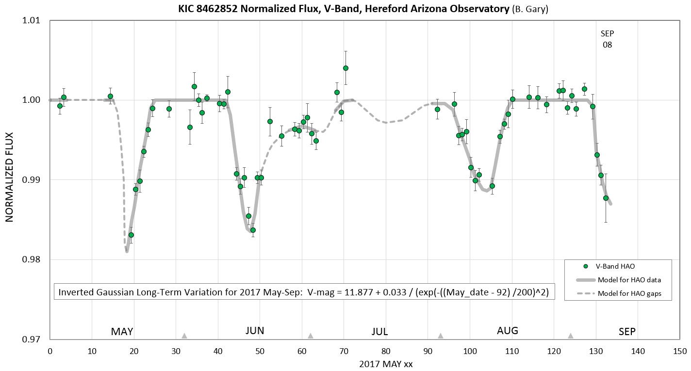
Figure 1.1. Light curve for "May
to now" for HAO V-band observations, with an adjustment for an
"Inverse Gaussian" model for the long-term variation/fade of OOT
brightness (Fig's 1.5 - 1.8 show that model). Only observing
sessions with at least 1.3 hours of observations above 30
degrees elevation and with mostly clear skies are included here.
Notice the different asymmetries for the three major fade
events: the May fade begins fast and recovers slower, the June
fade begins slower and its recovery is interrupted by a small
fade, while the August fade began slowly and recovered fast. I
don't know if the last observation's departure from the OOT line
is real; probably not.
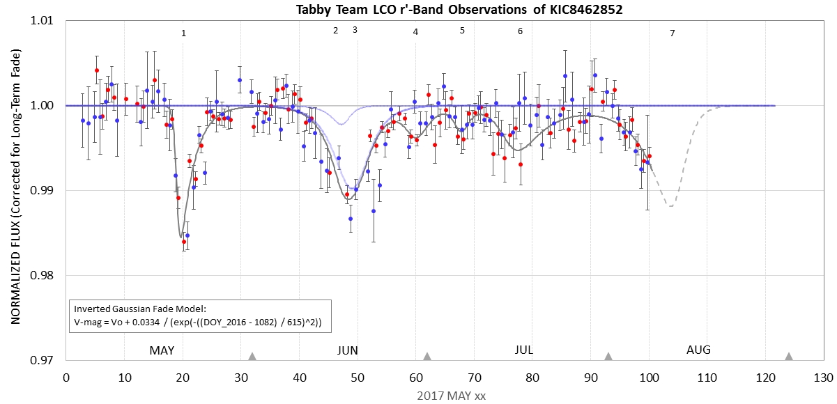
Figure 1.2. Tabby Team r'-band data (as of Aug 07),
graciously provided by Tabetha Boyajian to help in comparing
with HAO V-band observations. I have adjusted the Tabby Team
data for a
hypothesized long-term fade model (the "inverted
Gaussian" model, described below).
The gray trace is my fit to the data using 7 AHS components
(asymmetrical hyper-secant, used thousands of times for
fitting dust cloud dips exhibited by WD 1145+017, link1 & link2). The
AHS components #2 and #3 overlap, so their individual shapes
are show with dotted blue traces. The 7 AHS components have
been adjusted to provide a solution (minimum of
sum-of-chi-squares) for both the LCO r'-band data and
the HAO V-band data; the only exception is an additional
free parameter for multiplying depth of Dip#2 for
V-band. These r'-band data are from 16" telescopes at
the Las Cumbres Observatory sites in Hawaii (OGG) and
Tenerife (TFN).
The dip underway was at the ~ 0.7 %
depth level on Aug 7 (in agreement with the HAO data,
previous figure). I performed a sum-of-chi-squares minimization solution for all AHS
parameters (4 parameters for eqach AHS component, or dust
cloud). Comparing the above two figures
it is obvious that the dip in June ("Celeste") has a depth
ratio, D_r' / D_v, that differs from one. In fact, it is 0.24
(the Dip#2 r'-band depth is 1/4 of the V-band depth). This may
be due to the mid-May dip ("Elsie") being devoid of particles
smaller than 1 micron, while the early part of the mid-June dip
("Celeste") has an abundance of smaller than 1 micron particles.
(Could this be explained by the Elsie dust cloud being closer to
Tabby's Star than 0.2 a.u., with P = 30 days, whereas Celeste is
farther away? Nope! Must have another explanation.)
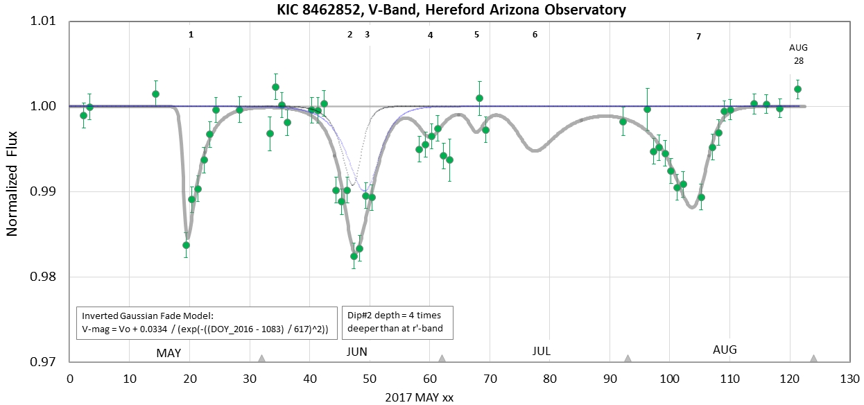
Figure 1.3. HAO V-band normalized flux, fitted with
AHS model that fits both the Tabby Team r'-band data and my
HAO V-band data, combined, allowing for only one difference:
the early part of the mid-Jun dip (Dip#2) has a depth that
differs from the r'-band depth. It is 4 times deeper for the
V-band data than the r'-band data. The August dip recovered
faster than it began, whereas the May fade began fast and
recovered slowly.
If the r'- and V-band data are accurate, then one could
tentatively conclude that Dip#2 has a particle size distribution
that includes small particles (smaller than 1 micron), whereas
there is no evidence for the presence of this component of small
particles for the other dips. Since I'm not that convinced of
the quality of all of this data I won't adopt that tentative
conclusion. So why did I go to the trouble of performing this
tedious analysis? To illustrate what I think should be done when
better data is available. (For example, maybe the Thatcher
Observatory V-band data is better than mine, or maybe some
professional astronomer has used a big aperture telescope to
monitor in two bands, and we don't know about those observations
yet - because that's what professional astronomers like to do.)
By the way, the AHS analysis for combined data sets at different
wavelengths has been done for WD 1145+017 in an article that has
just been submitted to MNRAS, and will soon be posted at arXiv
(Siyi et al). I'll give a link to the arXiv article when its
available.
How important is it to correct for long-term fade? There
are three reasons for this: 1) We don't know what's causing the
long-term fade (more accurately described as variations, just a
fade recently), so it's premature to assume that the cause is
dust, 2) even if the long-term variations are caused by dust they
are several "orders of magnitude" different in timescale (years or
decades vs. a few days) that their properties could differ
greatly, and therefore using the same parameters to describe them,
and solving for values, could be very misleading, and 3) whatever
the explanation for the long-term fade/variation when a dip occurs
we want to know about that specific dip's properties (i.e., depth
vs. wavelength dependence, as produced by the particle size
distribution of the particles in the dust cloud causing the dip).
Keep in mind that the current fade rate is well-established (by 3
observers), so adjusting for it does not strain objectivity. The
next figure is what Tabby sent me, which is uncorrected for
long-term fade (the long term variation is currently a "fade").
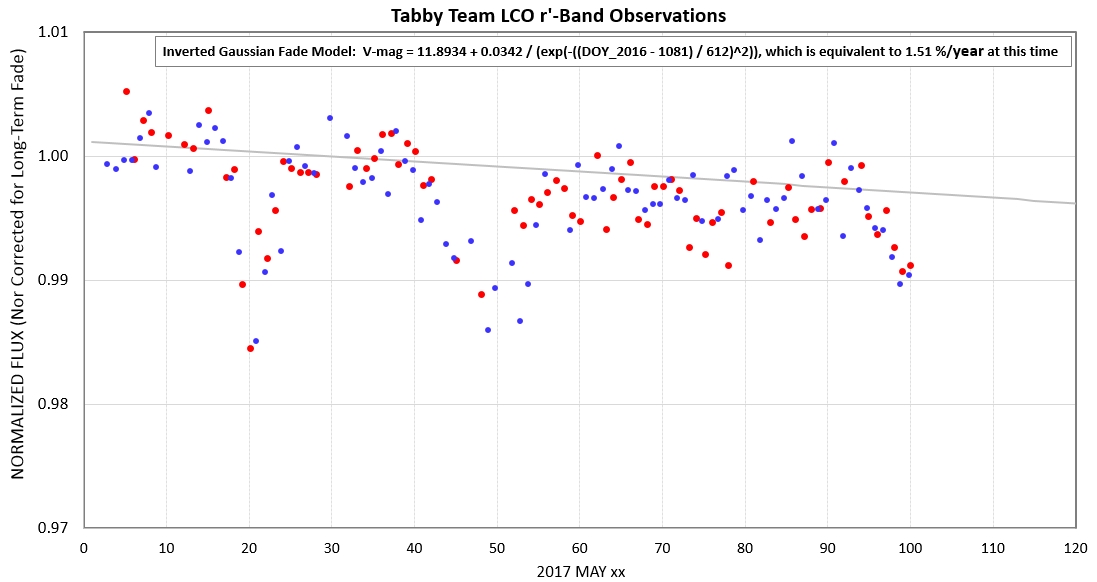
Figure 1.4. This is the Tabby Team r'-band data
provided to me by Tabby, on Aug 07. An "inverted Gaussian"
long-term fade model is superimposed (gray trace), since this
data doesn't allow for what I believe is a real OOT long-term
fade (shown in Fig's 1.4 - 1.6).
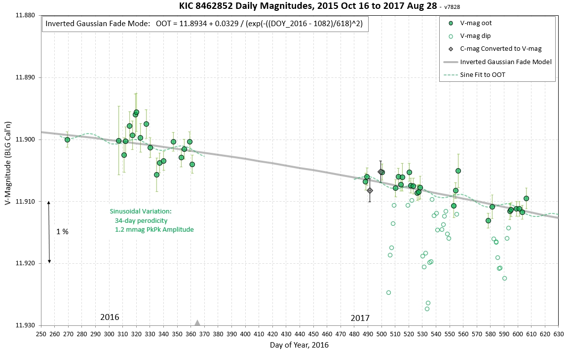
Figure
1.5.
These are my V-band observations from the past year,
plus some "clear filter converted to V-mag"
observations. Dip data are shown with open circles. An
"inverse Gaussian" long-term variation (fade)
model is shown (gray trace). Superimposed on the inverse
Gaussian model is a sinusoidal model that is marginally
statistically significant (at the ~ 5-sigma level). The
sinusoidal period is 34 days and peak-to-peak amplitude
is 1.2 mmag.
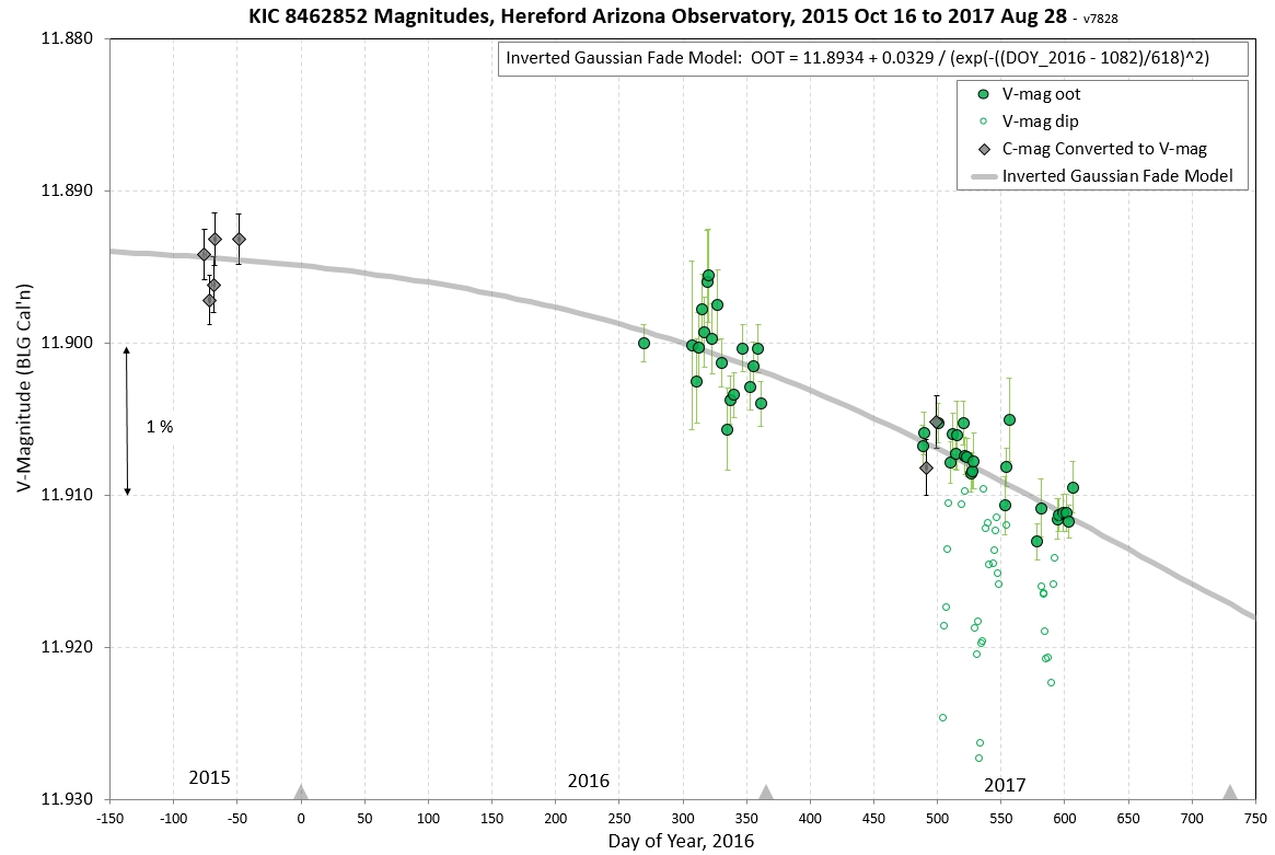
Figure 1.6. A 2-year span of observations showing the need
for a non-linear long-term variation (fade) model for
matching measurements that are judged to be "out-of-transit"
(OOT). Data taken during dips are represented by open circle
symbols. The gray trace is an "inverse Gaussian" model.(The
data within 300 < DOY_2106 < 360 exhibit a 29-day
sinusoidal variation with semi-amplitude = 2.9 mmag. With
only 2 cycles of coverage I hesitate to claim that such a
variation is real; more observations during an OOT state are
needed to confirm this possibly interesting finding.)
Is there independent evidence
for the long-term fade that I'm proposing? Yes, from two other
sources (the 2nd source is ASAS-SN observations, described in
the next section). The first data source confirming the HAO fade
during the past 1.5 years is from AAVSO data submissions by
David Lane (LDJ), shown in the next figure.
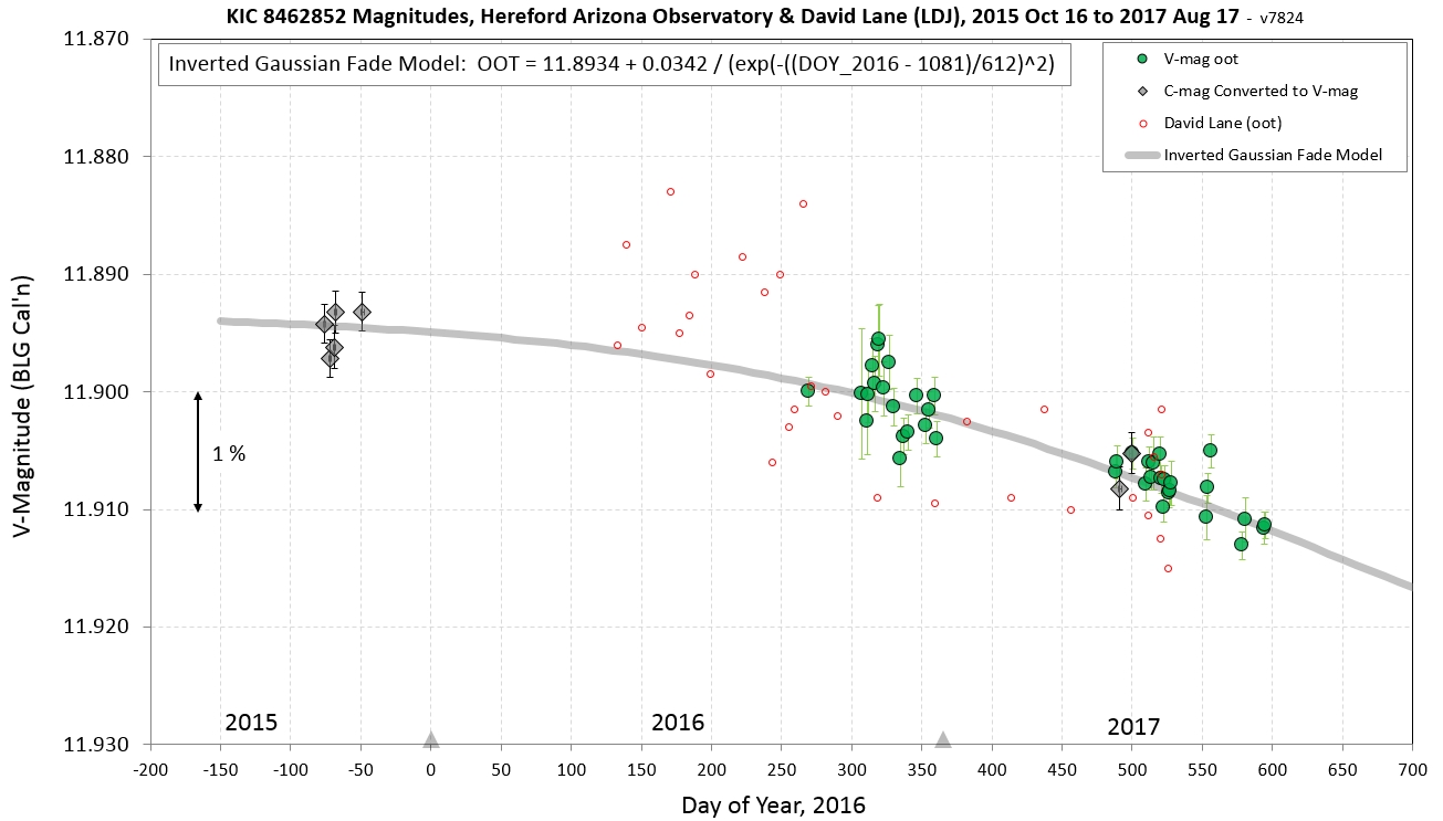
Figure 1.7. David
Lane's V-mag measurements (red circles) are superimposed
on the previous graph. Dip data have been omitted. An
offset of 0.07 mag was applied to the LDL data to
achieve empirical agreement (related to use of different
reference stars with different catalog V-mags). The LDL
data has been median combined in groups of 9.
The David Lane V-band
observations are not only compatible with the HAO V-band
measurements but they argue for the same long-term fade rate
for the interval where our two data sets overlap.
Note: If we adopt the 2015 magnitude
as the 100 % level for normalized flux, then the latest dip
would be at a normalized flux level of 97.5 % (i.e., depth of
2.6 %). I prefer to state that the dip is ~ 1.0 % below the
long-term fade level. As a future publication will show, the
non-dip brightness during the past decade is too variable to use
for establishing a reliable 100 % level; it just varies too
much! An additional reason for "correcting" a several-month long
LC for a best-estimate long-term fade model is that when this is
done it is possible to fit the dip structure using the AHS
model, as demonstrated in Fig's 1.2 and 1.3. Using AHS permits
other physical phenomena to be studied, such as which dips
exhibit unusual depth ratios (e.g., D_r' / D_v), which in turn
can be used for the interpretation of "particle size
distribution" differences between the different dust cloud dips.
That's why I suggest describing the dips as departures from the
long-term fade variations. ("That's my story, and I'm sticking
to it!")
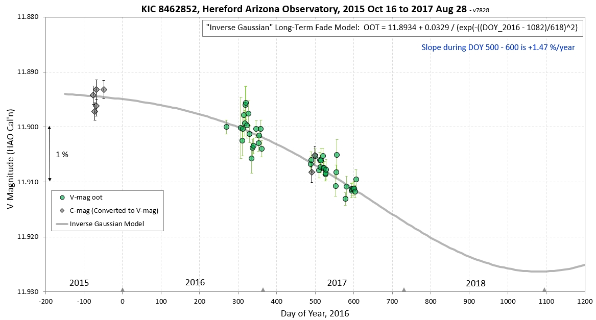
Figure 1.8. This 4-year light curve, with almost
2 years of data, is fitted with the
"inverted Gaussian" model.
The "inverted Gaussian" model is compatible with the
notion that brightness could level off next year (2018)
and begin to recover the following year (2019), eventually
returning to normal.
However, this is just an extrapolation of a mathematical
model, not based on a physical model, so extrapolating is
really unjustified. However, this behavior is what a dust
cloud model for explaining the long-term fade could
predict, as described by a plausible physical model
described below, link.
Of course, the model could only be an over-simplification
of the real situation, but it's a "guide" for what might
happen.
ASAS
Observations of Long-Term Variability
Joshua Simon et al. have published (link) 11
years of ASAS V-band observations, and 2 years of ASAS-SN
V-band observations (both using small ground-based
telescopes). These are the best quality long-term
monitoring observations (longer than the Kepler
4-year data set) so far of Tabby's Star.
The two V-mag series
agree where they overlap, and the ASAS agrees with the 4-year
Montet & Simon Kepler fade pattern. What's more
interesting, though, is year timescale brightenings in 2006/2007
and 2014. The latter was 4 %. During the last 2 years there's a
slow fade, consistent with my fade over the same time. With this
perspective I suggest that we can reinterpret the century of
DASCH data in the following way: decade timescale variations
with a peak-to-peak amplitude of 4 or 5 % could have been
occurring during the past century, but the DASCH data were
simply too noisy to have shown such variations. (The abrupt 0.12
mag shift in brightness, occurring across the infamous "Menzel
gap," is related to the change of plate emulsion and telescope
change that occurred at that time ~ 1960); therefore, we are
justified in discounting the suggestion (Schaefer, 2016) of a
century timescale "fade."
Simon et al. suggest that the 8-year
interval between brightening events of KIC846 might be evidence
for an 8-year variability due to a magnetic activity cycle. They
keep open the notion if interstellar medium structure since
their I-band LC shows long-term changes that are the same
(within the noise) as those for V-band; they recommend that
future monitoring projects include two bands to investigate
wavelength dependence of long-term brightness variations.
The most conservative
stance to take, I suggest, is that variations of as much as
5% occur on decade timescales. (Or, just because a 2-year
snippet shows a fade doesn't mean that Tabby's Star will
fade into oblivion, any more than a 2-year snippet showing a
brightening would mean that Tabby's Star will some day
outshine our sun.)
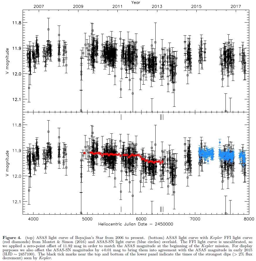
Figure 1.9. ASAS
V-band observations during the past 11 years (top
panel) with the Montet & Simon (2016) Kepler data
overlain (lower panel, red) and ASAS-SN data overlain (bottom
panel, blue). This figure was taken from
Simon et al. (2017).
Links Below
11-years of ASAS
V-band monitoring
Why
this web site
Basic Infor for
KIC846
Can
Structure Within an Observing Session be Believed?
List of Observations
Daily Observing
Session Details
Tutorial on
Fading Star Basics
Comparing
Kepler Data with Recent Data
Long
Term Trends
Plausible
Physical Model for Everything
A Prediction
References
Earlier Web
Page (#1) started 1.7 years ago, and no
longer updated
Why This Web Site?
This web page was started Jun 18 with the original
intention of avoiding the attention my observations were
getting at "reddit." I knew nothing about reddit until a
couple people e-mailed me in mid-June with incidental
mention that some people were criticizing my
observations. When I checked the reddit "thread" for
Tabby's Star I was initially unimpressed with the
quality of some of the postings, so that's when I
decided to discontinue daily updates of my KIC846 web
page (http://www.brucegary.net/KIC846/).
I intended this web page to be for my personal use.
However, after more than a dozen followers of the first
web page wrote to express their appreciation for my
observations, with a hope that I would change my mind
about discontinuing updates, I decided to give them the
URL to this web page. A few days ago someone pointed out
that the reddit thread was making frequent use of my
observations I took another look at the reddit
commentary, and was quite surprised to see frequent
reference to my observations. I also noted that some
postings were quite well-informed, and reasonable. I
have now decided to open this web page to the "public
domain." I'm aware that observations on this page will
somehow show up at reddit, and I am now OK with this.
By the way, I'm not a professional astronomer. I'm an
amateur, and I don't have any special background for
having an informed opinion about what is causing the
Tabby Star fades. My only qualification for contributing
to the Tabby Star mystery is experience in performing
quality photometry.
Basic
Info for KIC846
RA/DE =
20:06:15.5, +44:27:25
All-sky photometry: B = 12.493 ± 0.025, V =
11.912 ± 0.025, B-V = +0.581 ± 0.035, as
measured by B. Gary in 2016, link.
APASS Mag's: B = 12.360, V = 11.852 (B-V =
+0.51), g' = 12.046, r' = 11.697, i' =
11.554
There's
a 0.11 mag discrepancy between BV
mag's in Boyajian et al (Table 3)
and APASS (article is brighter).
There's a 0.23 & 0.21 mag discrepancy
between B & V mag's in Boyajian et al
(Table 3) and my all-sky V-mag (which are
fainter than Boyagian et al)
Distance (based on Boyagian et al V-mag) is
1480 light years (454 pc).
Star Teff = 6750 K. Star radius = 1.58 x Rsun
Rotation period = 21.11 hrs (but should vary with
latitude).
Brown dwarf (?) star 1.96 "arc (900 a.u.) to east. Too
far to be gravitationally important now (but we don't
know its past path)
Question: How do my
HAO observations compare with the Tabby Team Las Cumbres
Observatory observations?
Consider the following two figures.
3. Can
Structure Within an Observing Session be Believed?
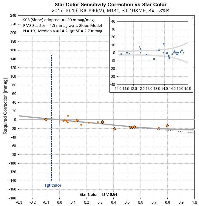
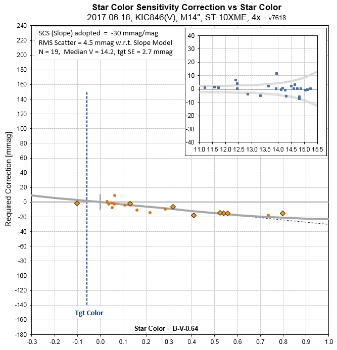
Whereas
the process of using reference stars to provide a magnitude
calibration for an observing session may be subject to an
uncertainty of 3 mmag (0.3%), for example, all observations
within the observing session may share the same systematic
error and therefore provide other information, such as slope
within the observing session. If such a slope within an
observing session can be trusted then we would have additional
information that could be used to create an improved model for
what was happening between observing sessions. I have
attempted to make use of this slope information in creating
the following figure.
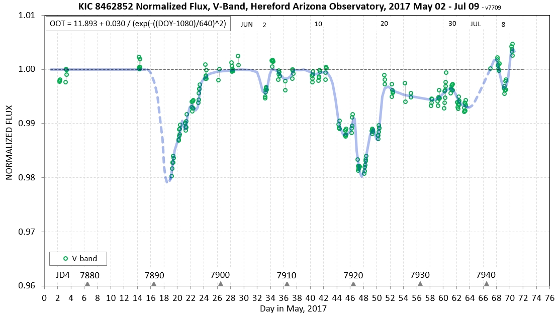
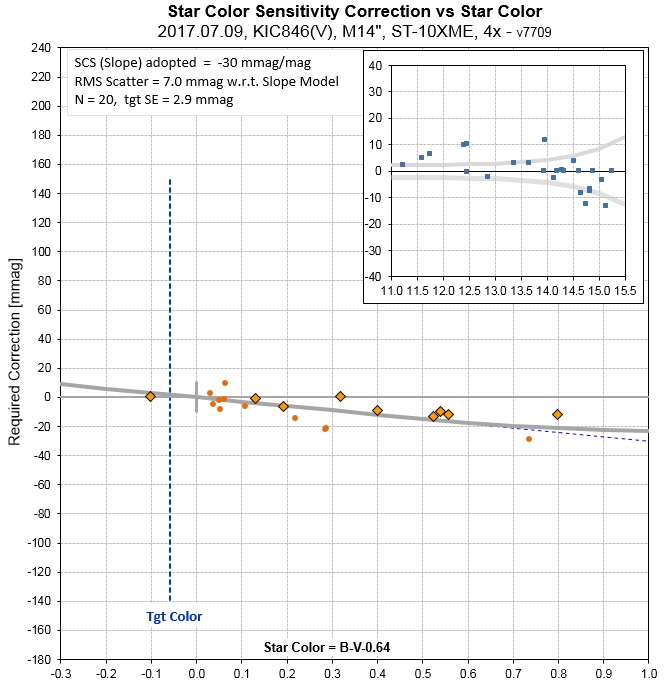
Figure 3.1. This
2-month light curve is modeled in a way that makes use of
information about the slope of brightness within observing
sessions.
At this time I do not know whether to trust slopes in this
way. It should be kept in mind that the overall level of each
observing sessions measurements is expected to be uncertain at an
estimated 0.3 % level for good observing conditions, and up to ~
0.4 % for poor observing conditions - as the following analysis
shows.
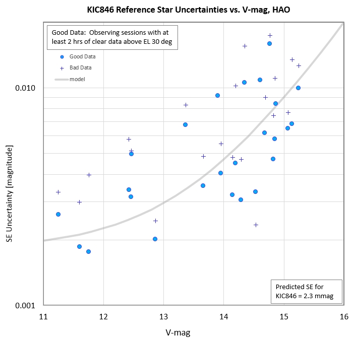
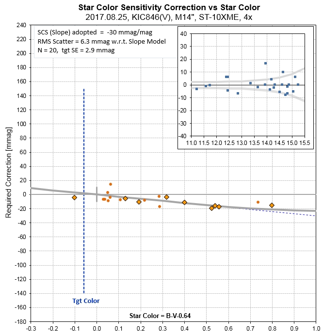
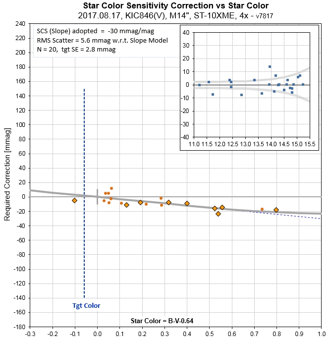
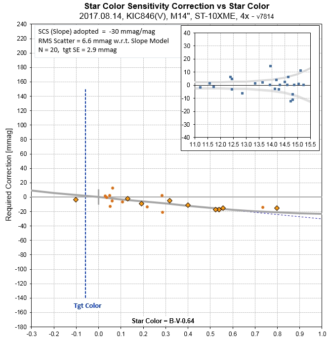
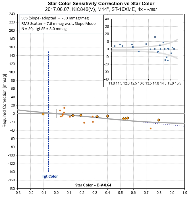
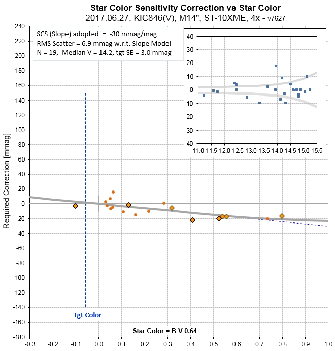
Figure 3.2 "Good" and "bad" observing sessions
exhibit different uncertainties vs. reference star brightness. A
"good" observing session has at least 2 hours of clear weather
observations above 30 degrees elevation, while "bad" observing
sessions have less than 2 hours of good observing (some have
clouds throughout the session). Among the 40 observing sessions
in this analysis 30 are "good" and 10 are "bad." The model fit
is for the "good" observing sessions and it has two components:
1) "stochastic uncertainty," that depends on signal-to-noise
level, and 2) "systematic error," which is a fixed value (i.e.,
the same for all stars). The model is a sum of both components.
Since KIC846 has V-mag ~ 11.9 it is predicted to exhibit total
uncertainty (stochastic plus systematic) of ~ 2.2 mmag (or 0.22
%).
At the present time I don't know how
much to believe about the normalized flux trends within an
observing session, when uncertainties should be mostly
"stochastic" (with systematics shared for all data). Here's an
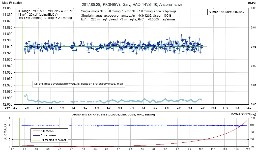
example of internal consistency at the 1.0 mmag level. Since it is
for one of my best observing sessions I think it can serve as a
lower limit on level of variations that can be searched for as
possibly real: namely, 1.0 mmag or 0.1 % of normalized flux.
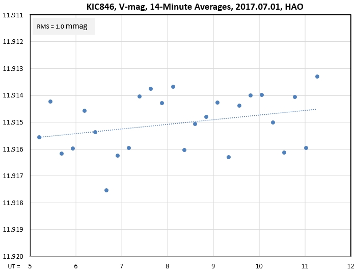
Figure 3.3.
Internal consistency during an observing session, suggesting
that variations of 14-minute averaged data exhibit an RMS
uncertainty of 1.0 mmag (0.1 % of normalized flux).
If this argument is valid, then the following light curve segments
(showing 1-hour averages, with an expected SE of no better than
0.5 mmag, or 0.05 %) may be worth considering.
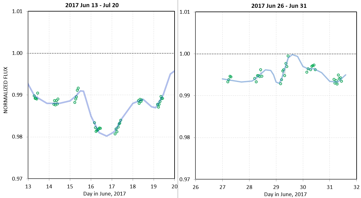
Figure 3.4. Expanded date scales for two date regions,
showing possible model fits that involve short
timescale variations. It's too early for me to be "a believer."
List of Observations (for all earlier observations, before Jun 18, go
to link)
2017.08.28 V
2017.08.25 V
2017.08.23 V
2017.08.21 V
2017.08.17 V
2017.08.16 V
2017.08.15 V
2017.08.14 V
2017.08.12 V
2017.08.09 V
2017.08.08 V
2017.08.07 V
2017.08.06 V
2017.08.05 V
2017.08.04 V
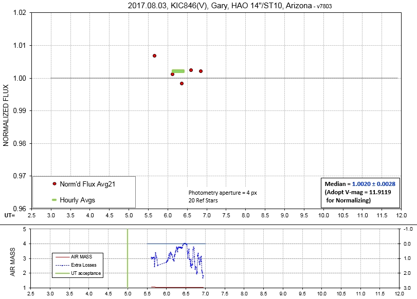
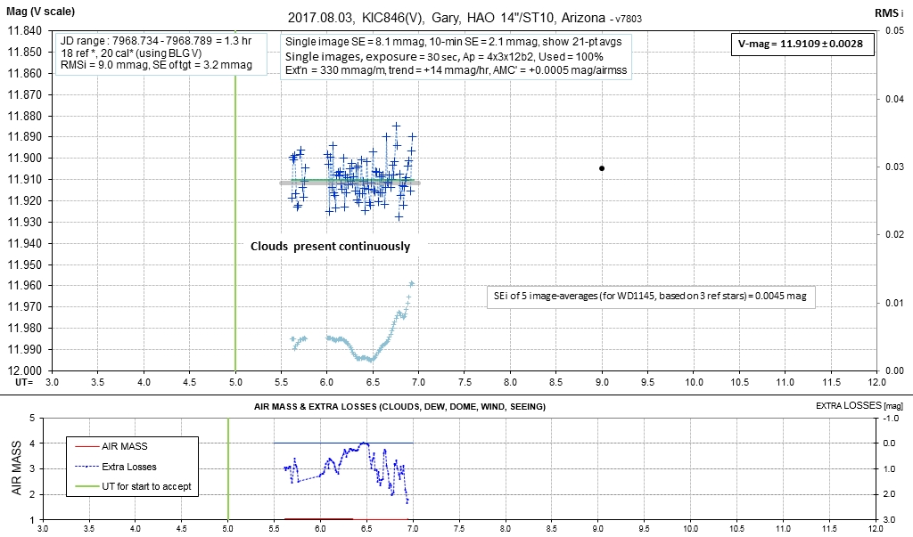
2017.08.03 V
2017.07.31 V
2017.07.09 V
2017.07.08 V
2017.07.07 V
2017.07.06 V
2017.07.02 V
2017.07.01 V
2017.06.30 V
2017.06.29 V
2017.06.28 V
2017.06.27 V
2017.06.24 V
2017.06.23 V
2017.06.21 V
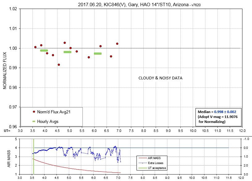
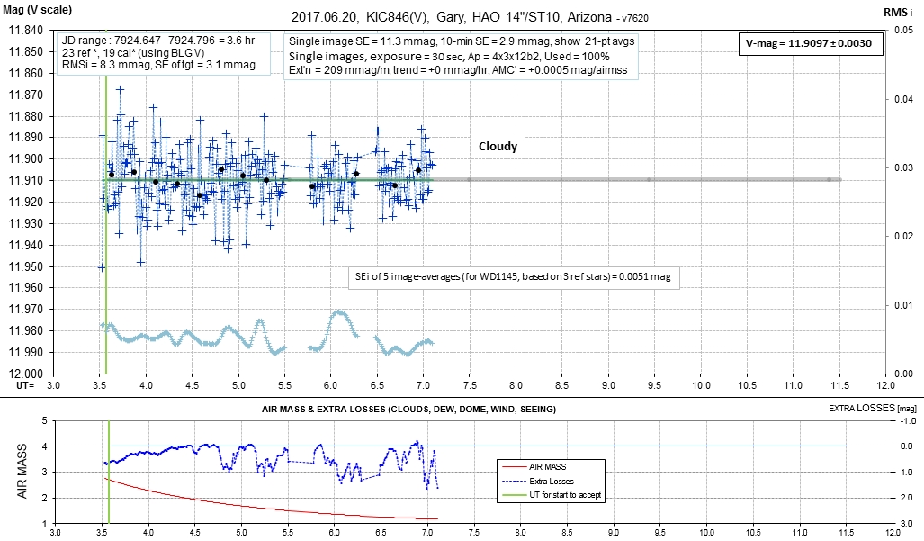
2017.06.20 V
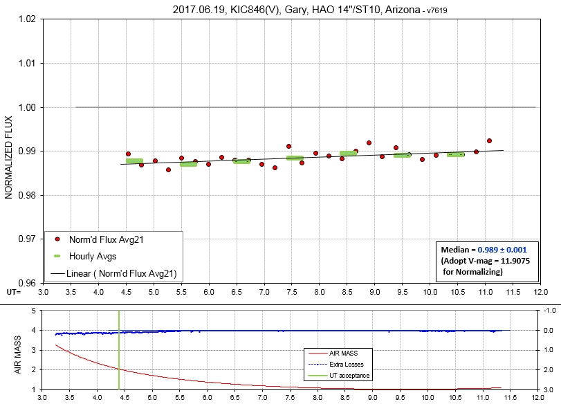
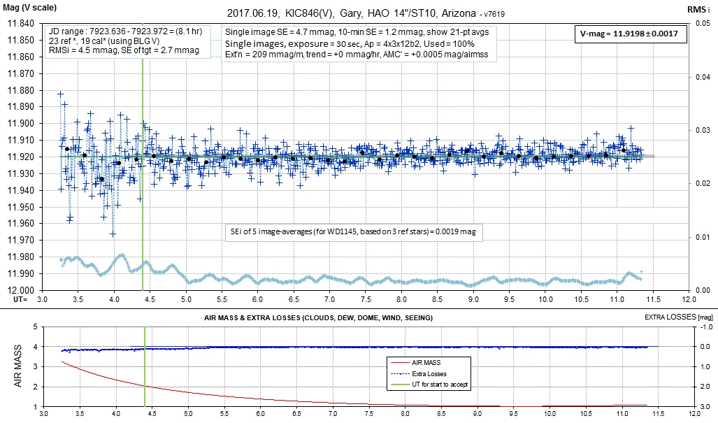
2017.06.19 V
2017.06.18 V
Daily Observing
Session Information (most
recent at top)
2017.08.28, V-band, 7.5 hrs of useful
data DataExchangeFile
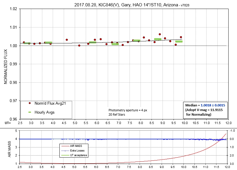
It's a little concerning that as noise level rises, which is
probably due to air mass increasing, the brightness also
increases.
I didn't use data after10.0 UT, when air mass rose above 2.0,
because I didn't want noisy data to "contaminate" better
quality data.

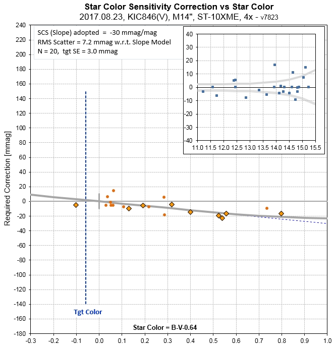
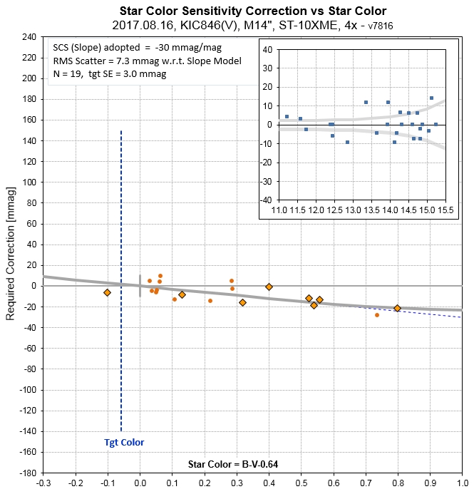
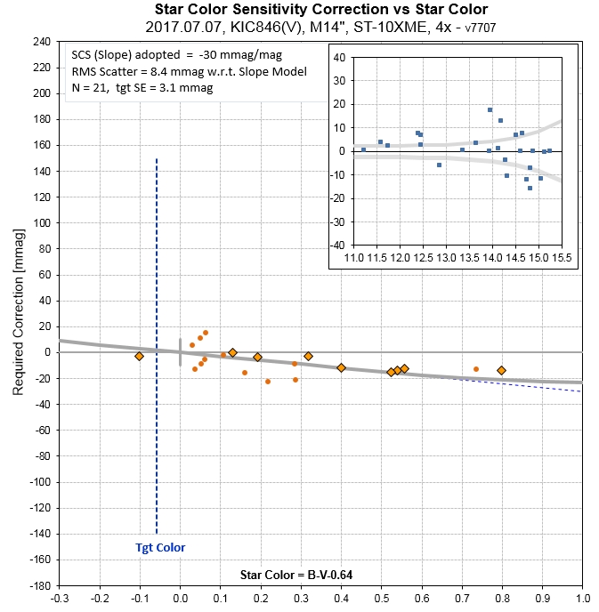
The bluest reference star is consistently "below" the model fit
trace. This just means that it could use a fine
adjustment of ~ 5 mmag for its adopted V-mag. I won't do it
because then I'd have to reprocess all previous LC sessions.
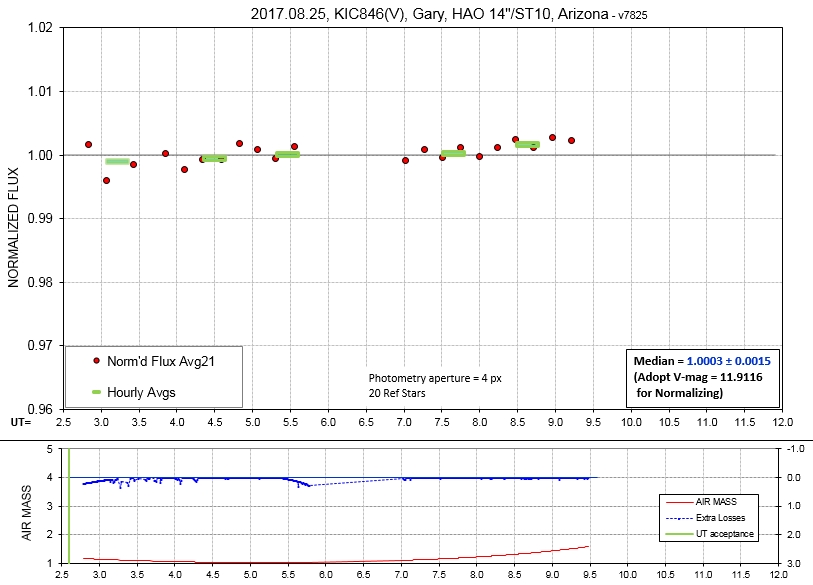
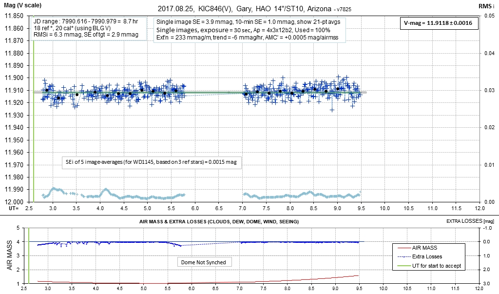
2017.08.25, V-band, 8 useful hrs, DataExchangeFile
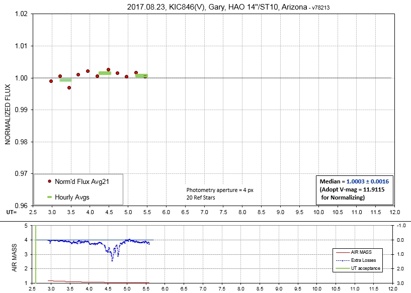
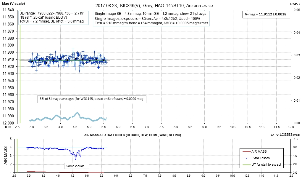
2017.08.23, V-band, 2.7 hrs, DataExchangeFile
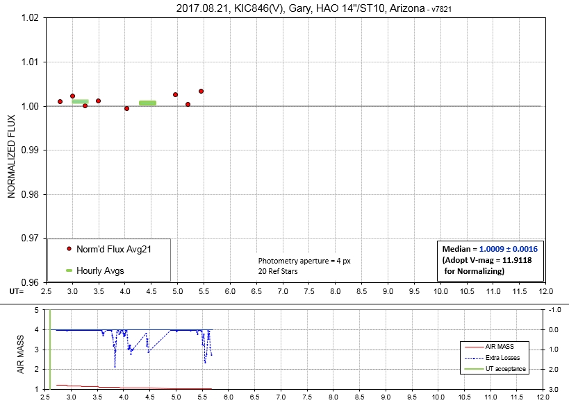
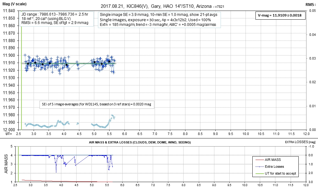
2017.08.21, V-band, 2.5 useful
hrs, DataExchangeFile

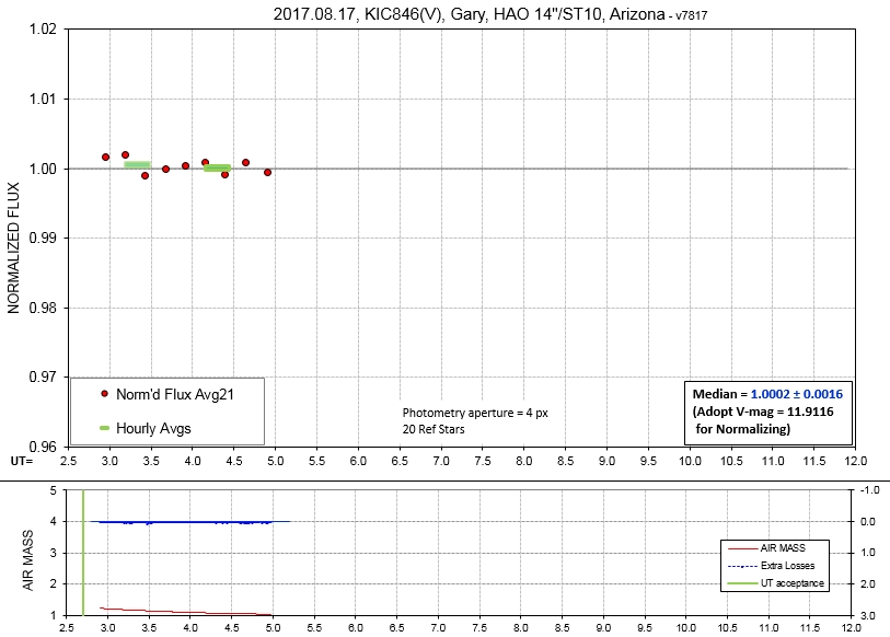
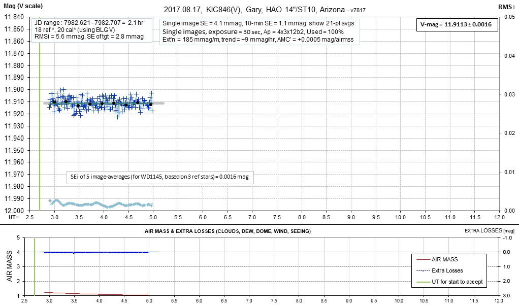
2017.08.17, V-band, 2.1 hrs
DataExchangeFile
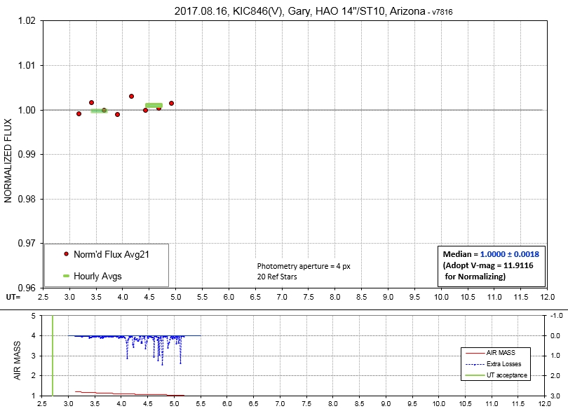
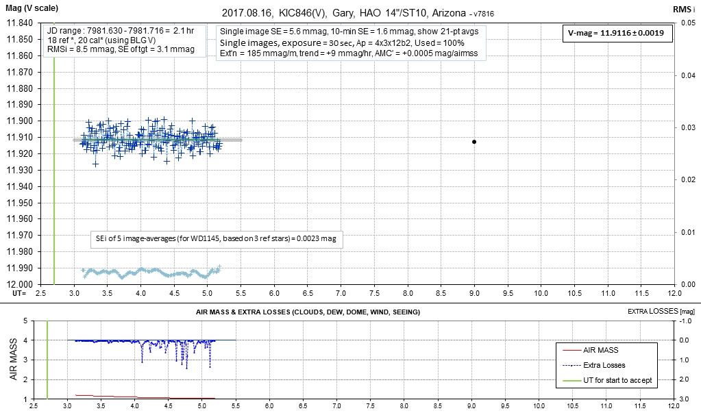
2017.08.16, V-band, 2.1 hrs, DataExchangeFile
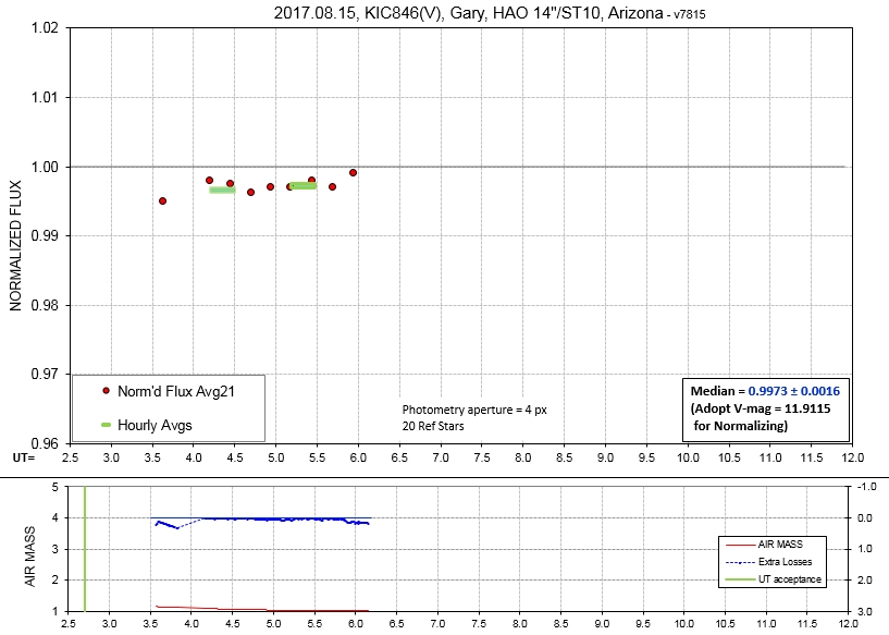
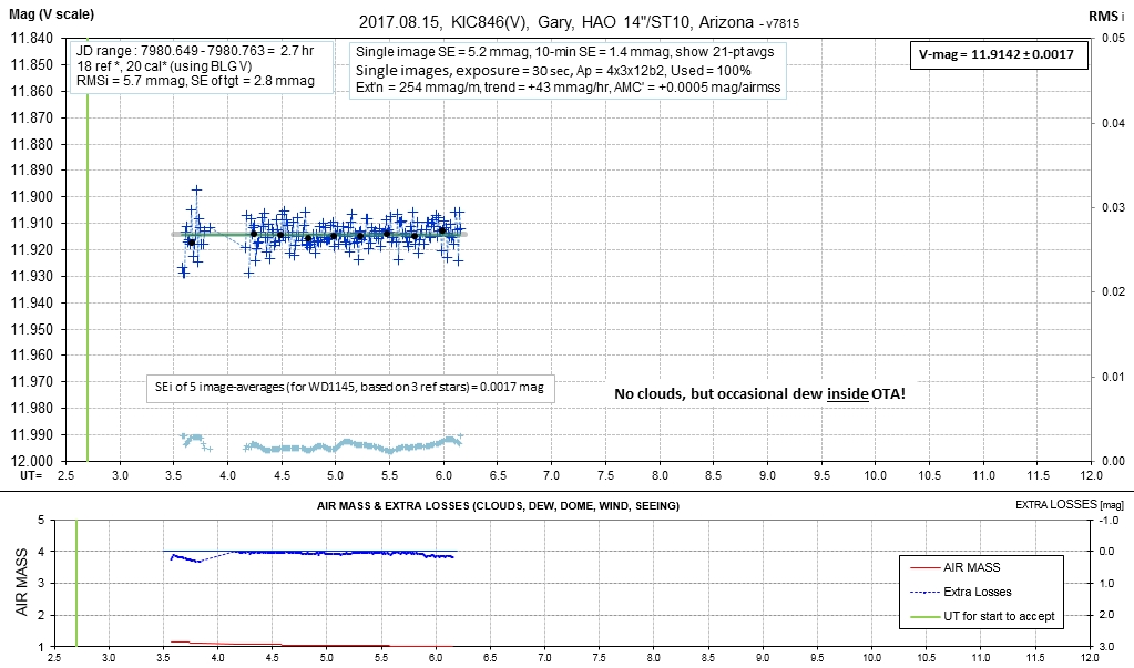
2017.08.15, V-band, 2.5 hrs useful
data, DataExchangeFile

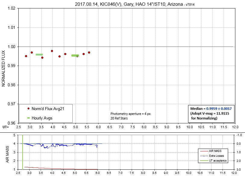
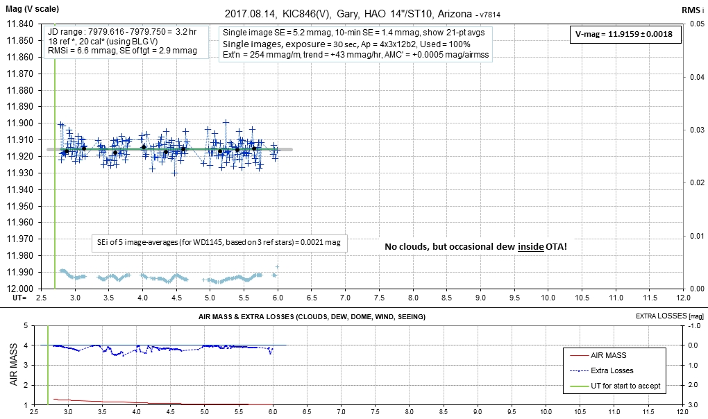
2017.08.14, V-band, ~ 3 hrs DataExchangeFile
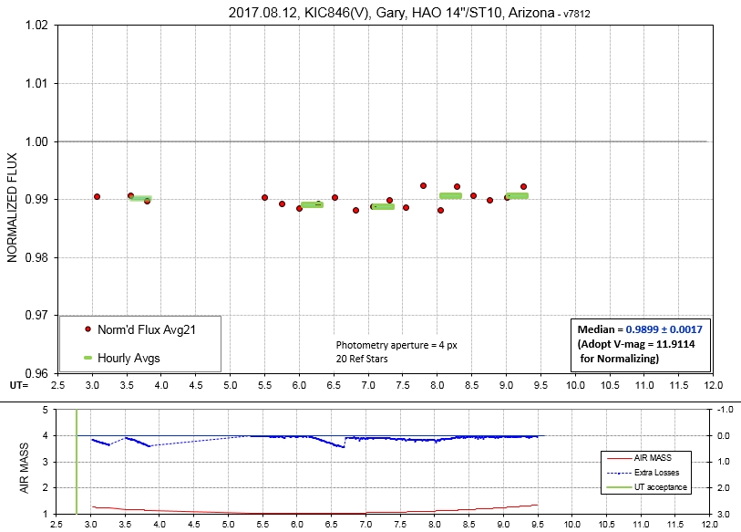
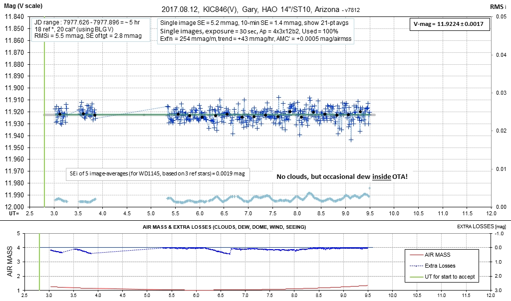
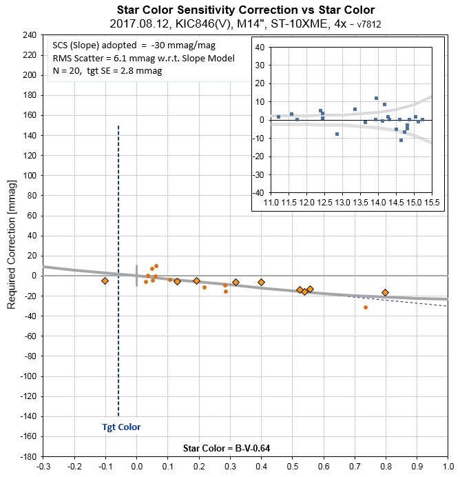
2017.08.12, V-band, ~ 5.0 useful
hrs, DataExchangeFile
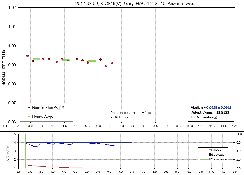
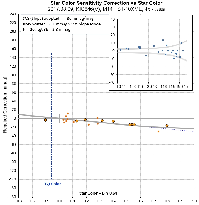
2017.08.09, V-band, 3.9 hrs, DataExchangeFile
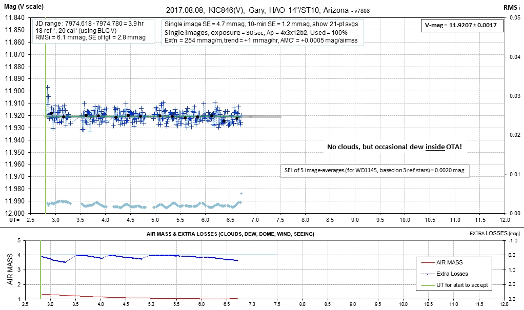
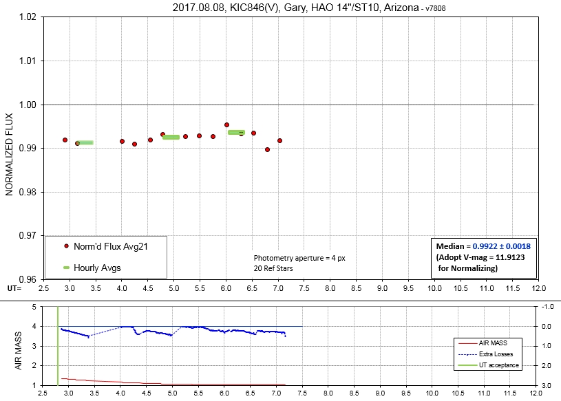
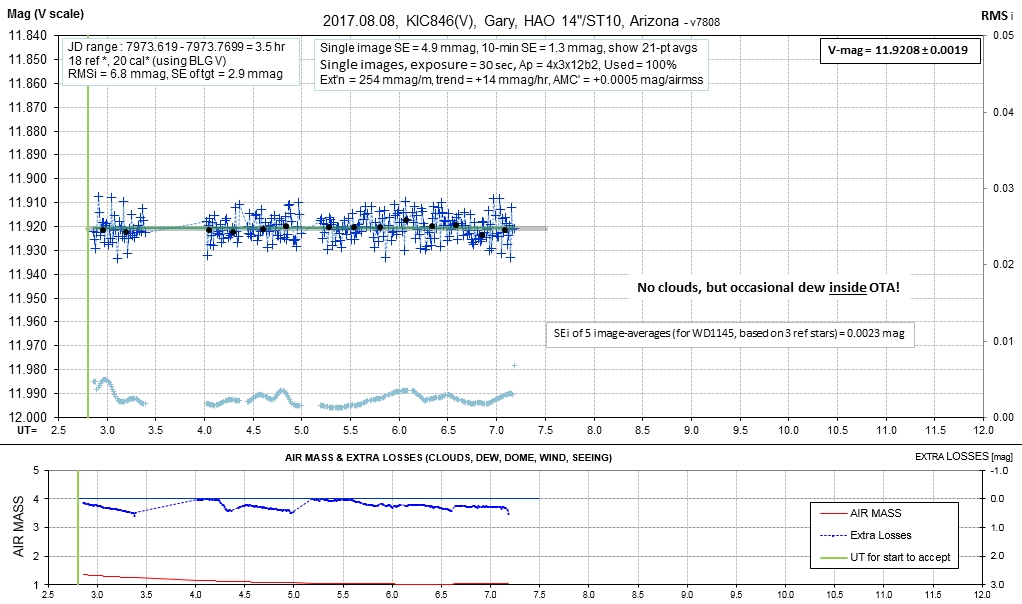
2017.08.08, V-band, 3.5 useful
hrs DataExchangeFile
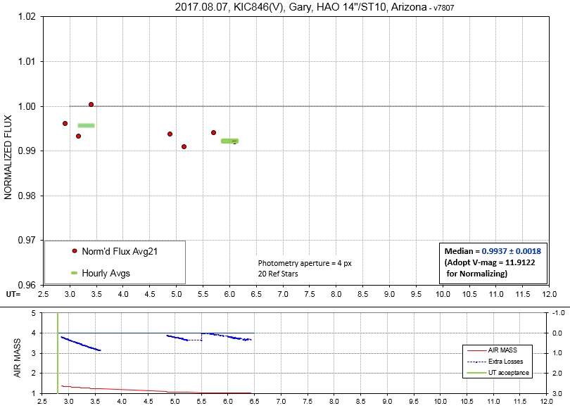
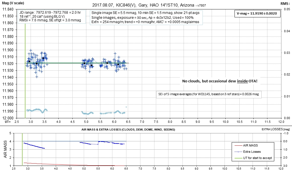
2017.08.07, V-band, 2.0 hrs of useful
data DataExchangeFile
I had to "dry out" the inside of my (closed tube) telescope twice
to evaporate water condensation on the corrector plate. This
problem will eventually go away, but only when ambient water vapor
dew point goes significantly below its current 60 F.
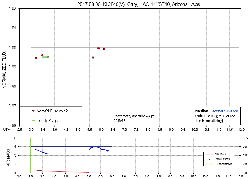
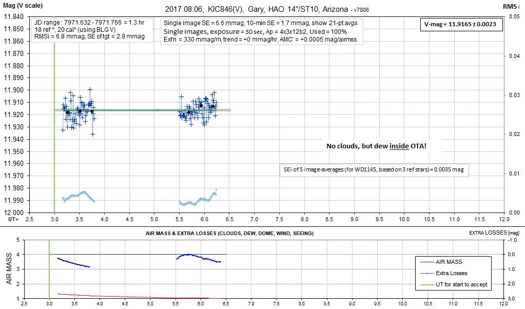
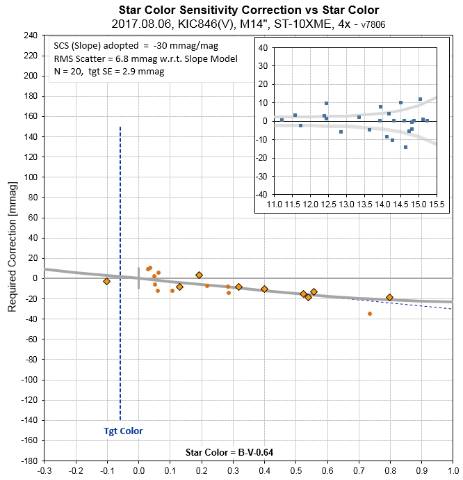
2017.08.06, V-band, ~ 1.32 useful
hrs, DataExchangeFile
Although the sky was clear, the high humidity during the past few
weeks raised the amount of water vapor inside my telescope tube so
much that when the optical surfaces cooled tonight they frosted
over with dew. I used a hair dryer to evaporate dew from the
corrector plate but then the water vapor condensed on the primary
mirror!
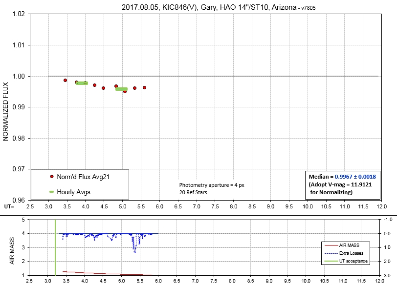
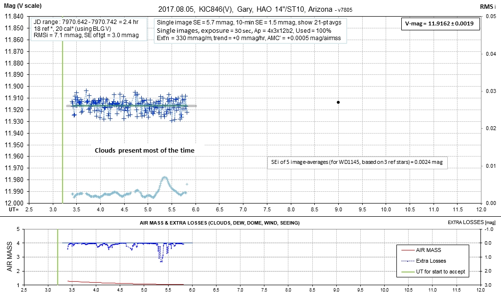
2017.08.05, V-band, 2.4 hrs, DataExchangeFile

2017.08.04, V-band, ~5.0 hrs, DataExchangeFile
The observing session was plagued by clouds, but during clearings
there was a consistent normalized flux of ~ 0.3 % below OOT level.
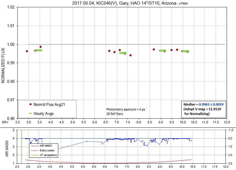
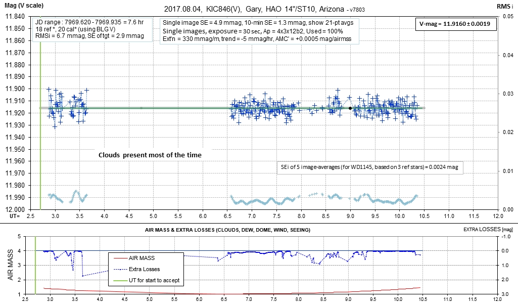

This calibration looks OK, i.e., unaffected by
intermittent cloudiness.
2017.08.03, V-band, 1.3 hrs
DataExchangeFile
I was "desperate" to observe, so when a "sucker hole" opened up, I
opened my observatory. Take this observing session result "with a
grain of salt."
It would be my opinion that a new dip is not underway.
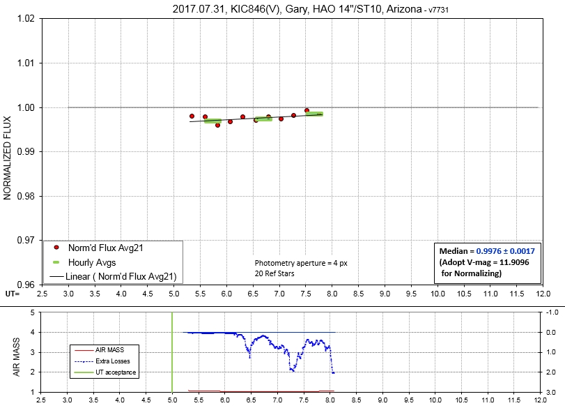
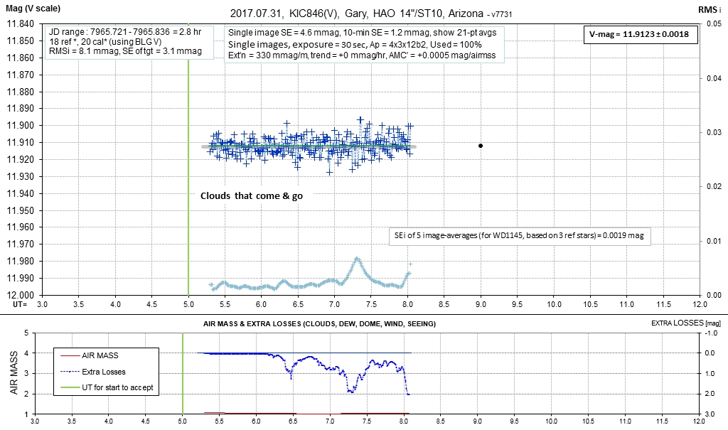
2017.07.31, V-band, 2.8 hrs
DataExchangeFile
Either KIC846 still hasn't recovered, or my long-term fade model
is under-estimating the fade acceleration!

2017.07.09, V-band, 4.4 hrs (of usable
data) DataExchangeFile
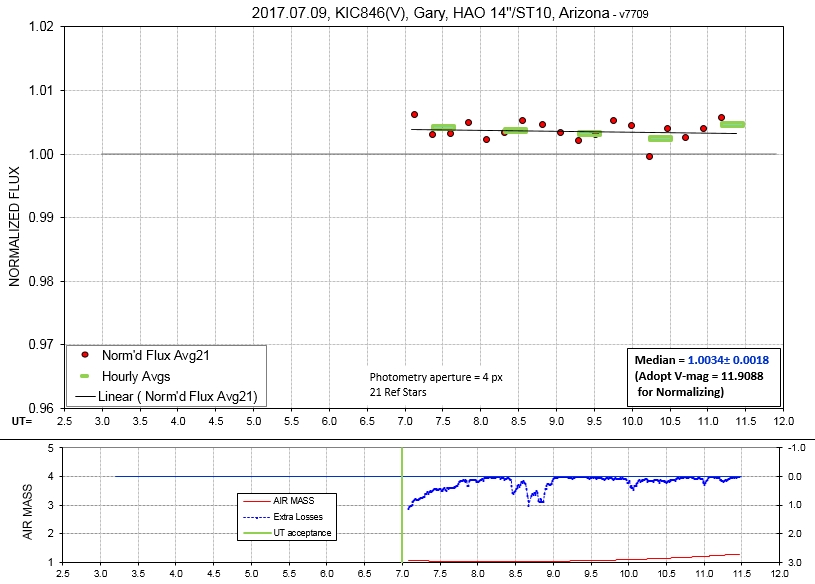
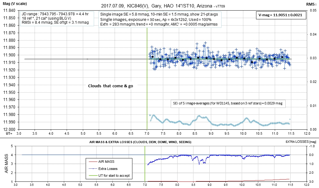
Clody until midnight, then partly cloudy.
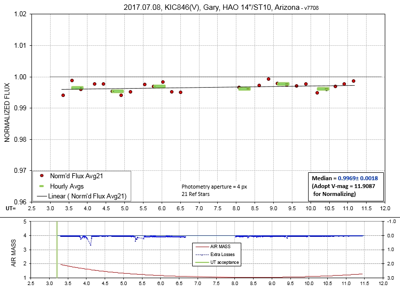
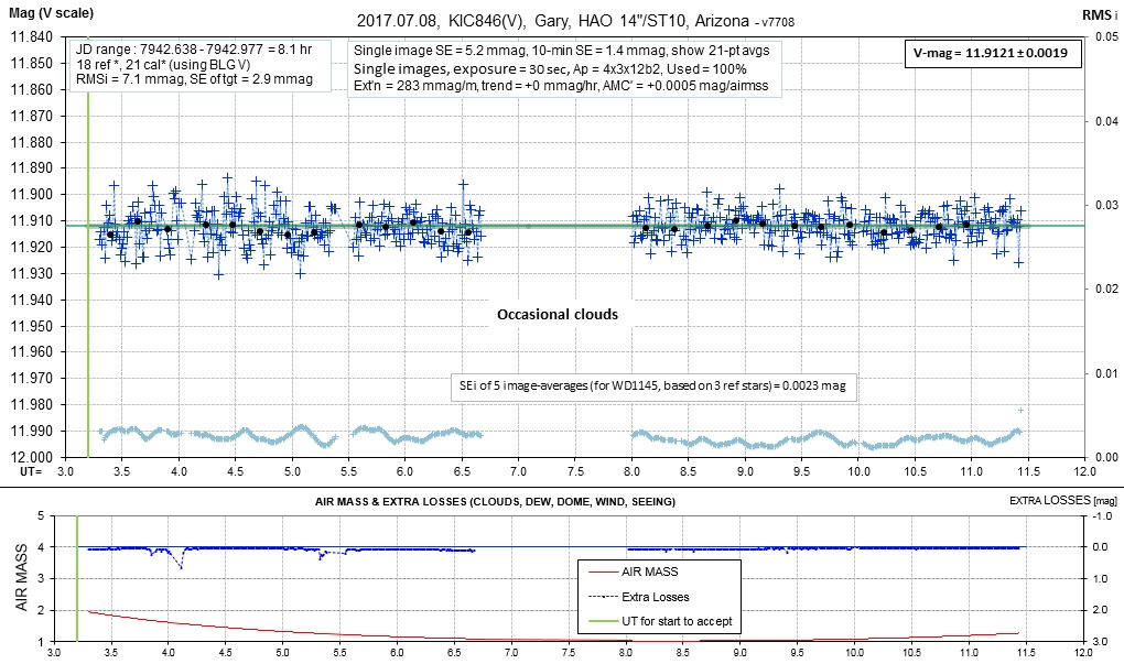
2017.07.08, V-band, 8.1 hr
DataExchangeFile

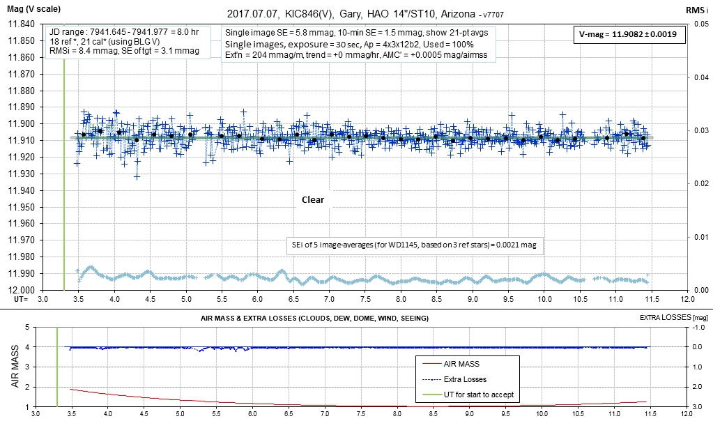
2017.07.07, V-band, 8.0 hr DataExchangeFile
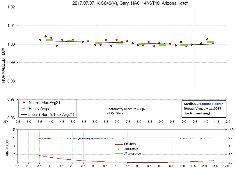
I don't know if the downward slope is real.
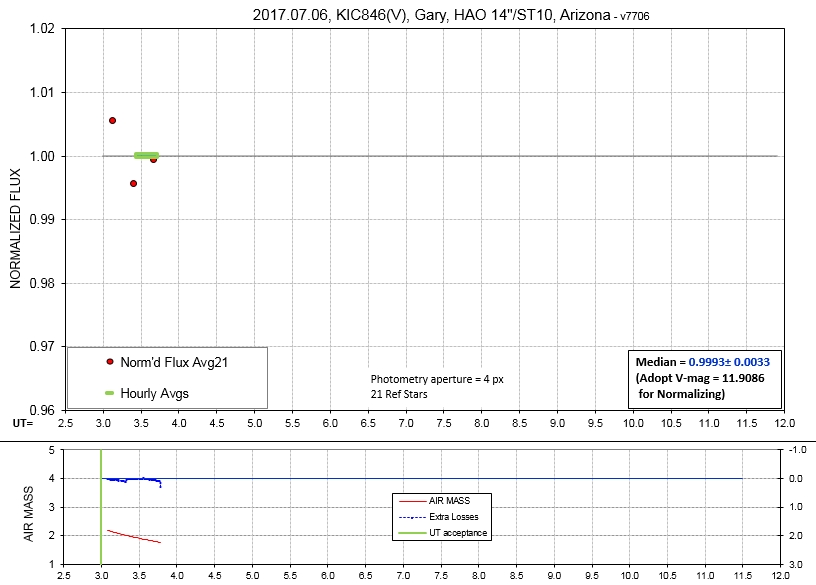
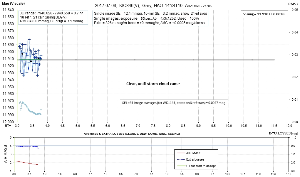
2017.07.06, V-band, 0.7 hr
I was desperate for a measurement, so I observed just before a
thunderstorm arrived.
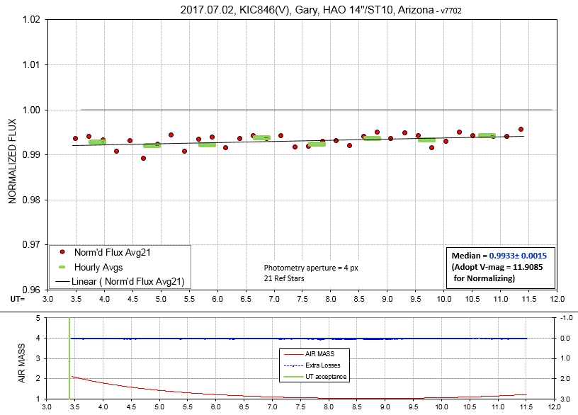
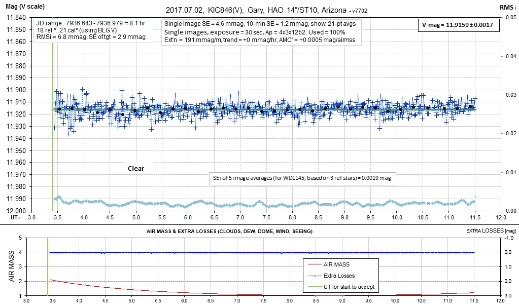
2017.07.02, V-band, 8.1 hrs, DataExchangeFile
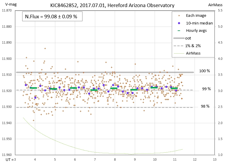
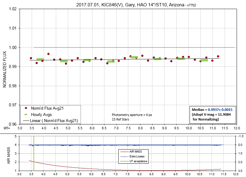
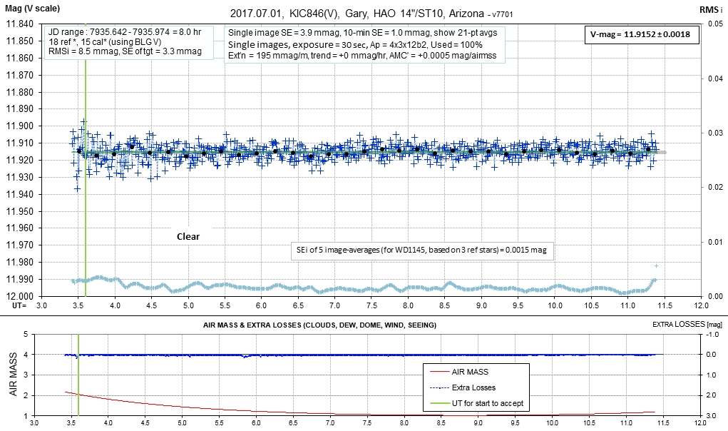
2017.07.01, V-band, 8.0 hrs DataExchangefile
Averages of 14 minutes exhibit an RMS scatter of 1.0 mmag. (I
want to thank Rafik Bourne, or Perth, Australia, for studying
my "data exchange file" magnitudes and prompting me to
identify outliers and rely more on better quality observing
sessions. This graph, showing millimag scatter, was one of his
suggestions.)
The two processing methods disagree by 0.3%. I'm concerned
about this and will continue to investigate.
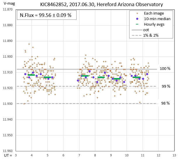
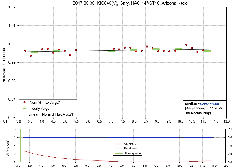
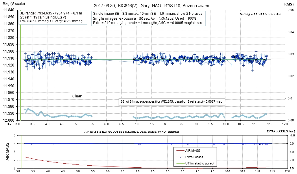
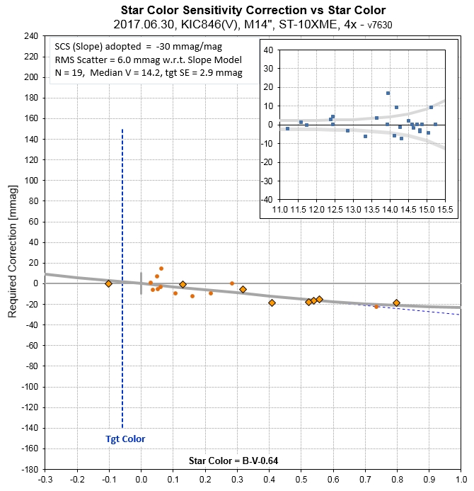
2017.06.30, V-band, 8.1 hr DataExchangeFile
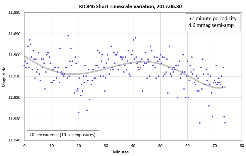
During 1.2 hours I took 10-sec exposures, unfiltered, which
show a 52-minute periodicity with a semi-amplitude of 4.6 mmag.
This short-term variation is similar to what I measured 1.7
years ago; I measured a 49-minute variation with 1.8 mmag
semi-amplitude: link
New data product: differential photometry using 7 "same color"
reference stars.
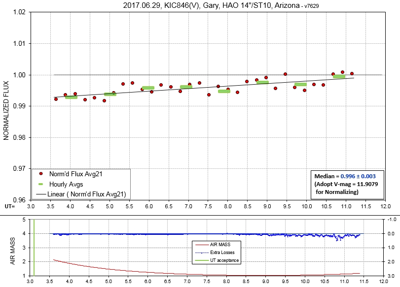
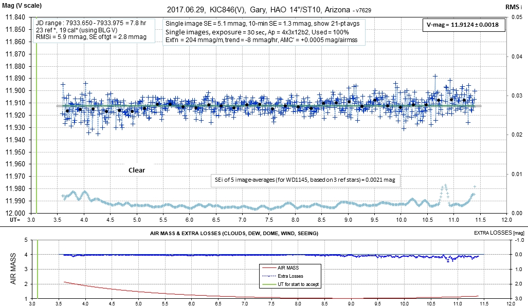
2017.06.29, V-band, 7.8 hrs DataExchangeFile

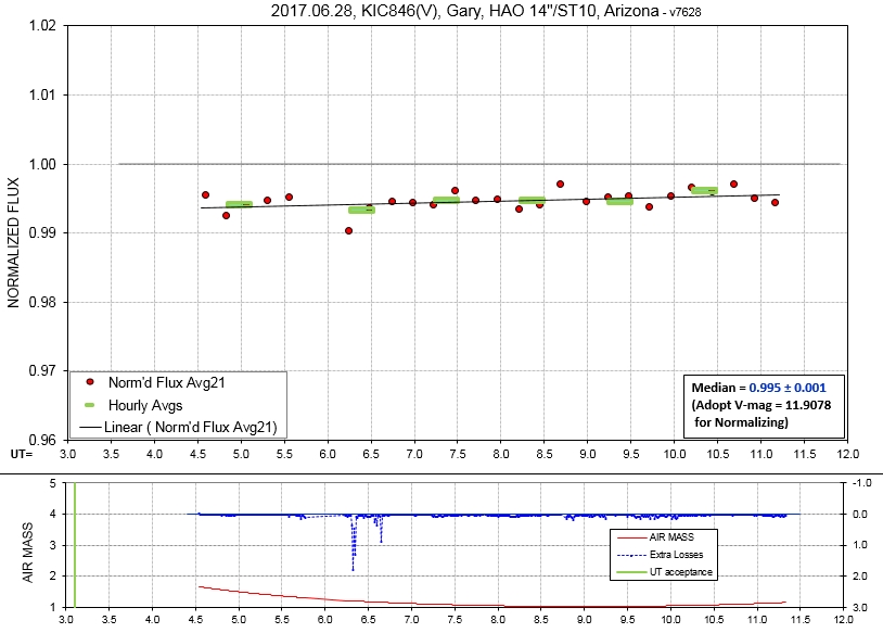
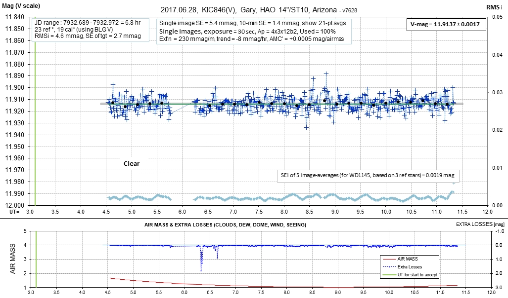
2017.06.28, V-band, 6.8 hrs DataExchangeFile

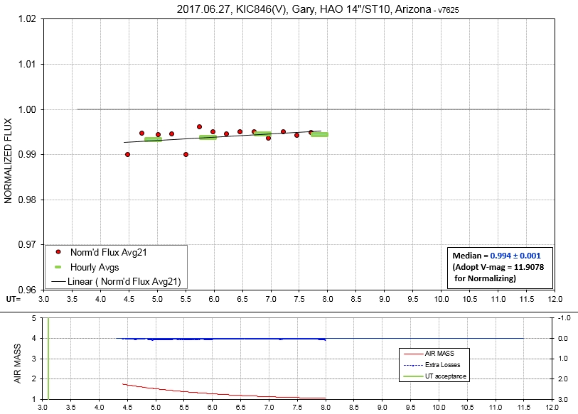
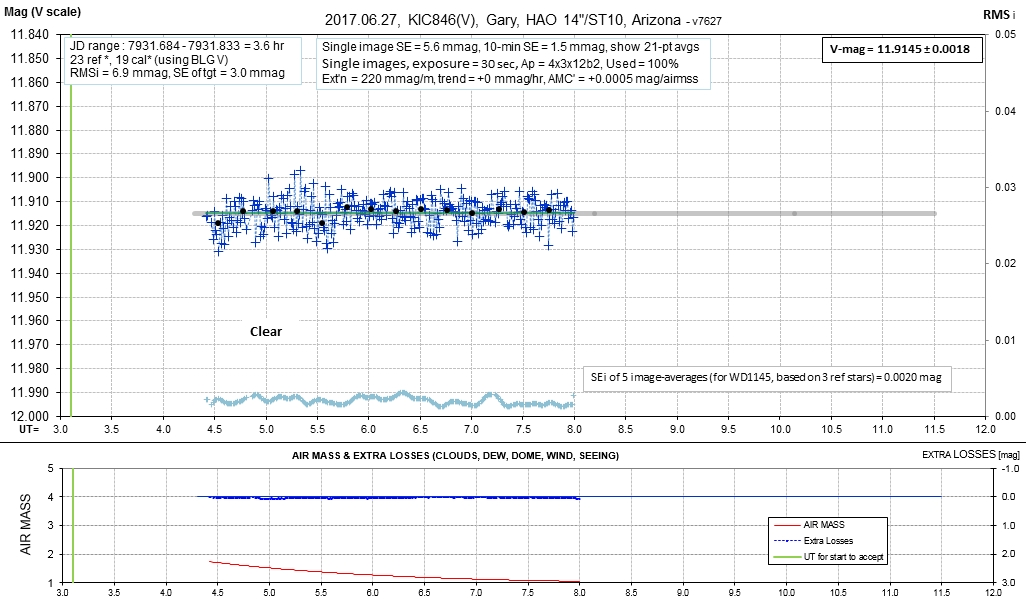
2017.06.27, V-band, 3.6 hrs, DataExchangeFile
2017.06.24, V-band, 2.2 hrs, DataExchangeFile
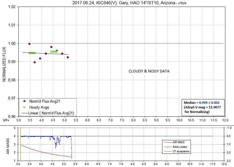
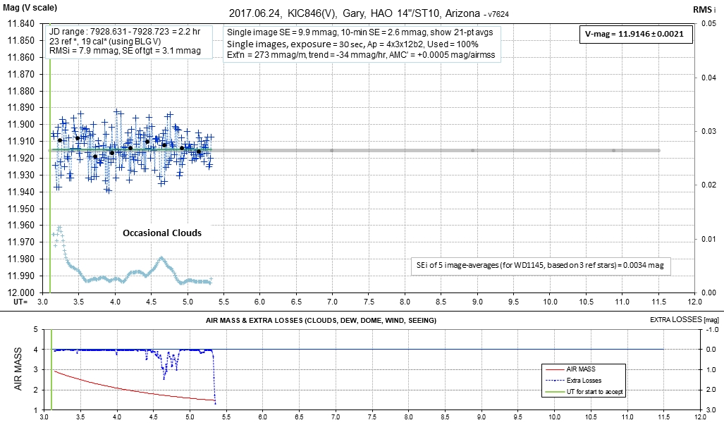
Thick clouds ended observing session.

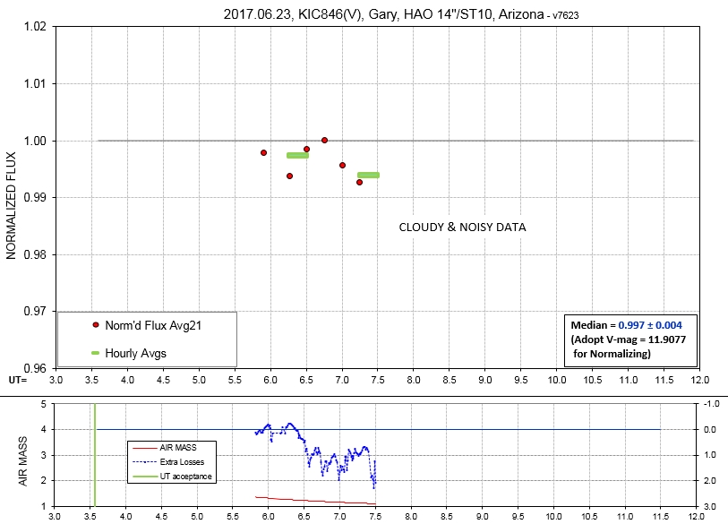
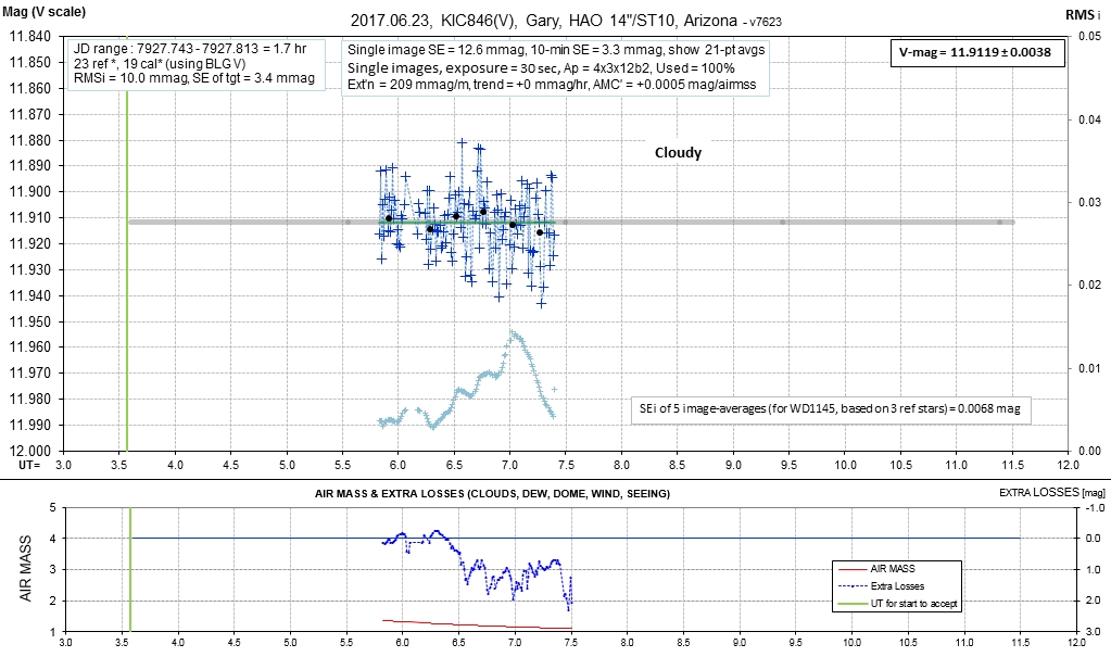
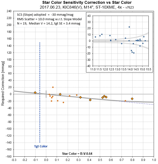
2017.06.23, V-band, 1.7 hrs, DataExchangeFile
Cloudy the entire observing session (up to 2.0 mag of loss), so
data quality is poor.
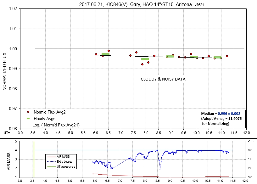
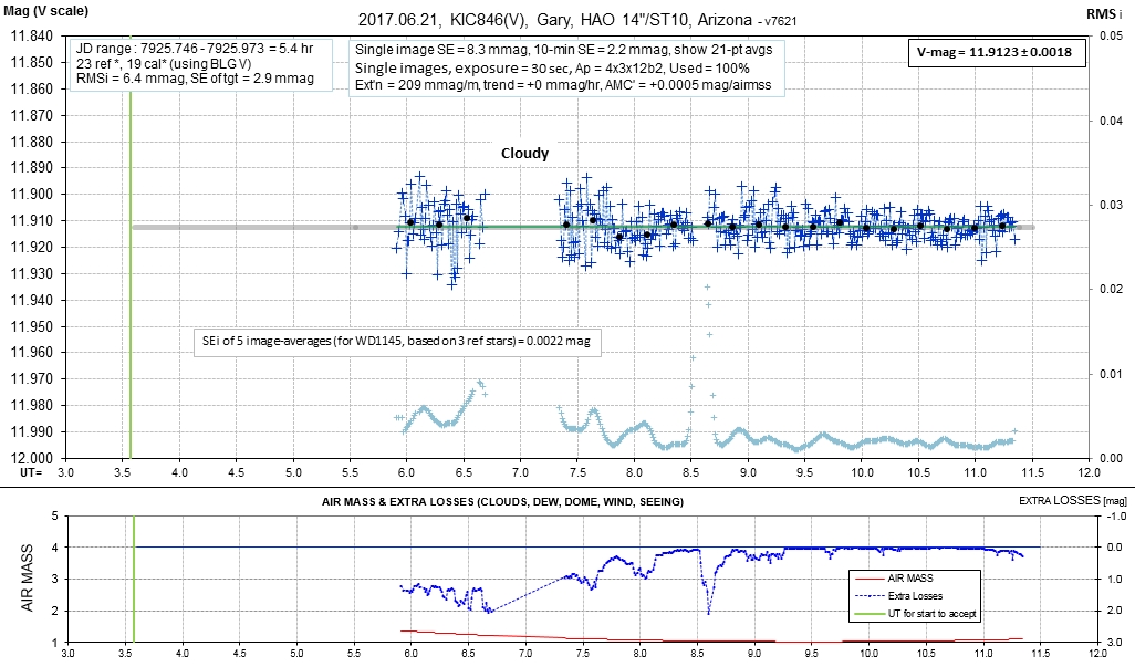
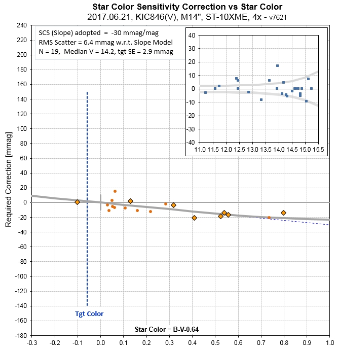
2017.06.21, V-band, 5.4 hrs DataExchangeFile
Skies cleared at midnight, so I got ~ 5 hrs of acceptable images.
2017.06.20, V-band, 3.6 hrs DataExchangeFile

2017.06.19, V-band, 8.1 hrs, DataExchangeFile
2017.06.18, V-band, 5.1 hrs, DataExchangeFile
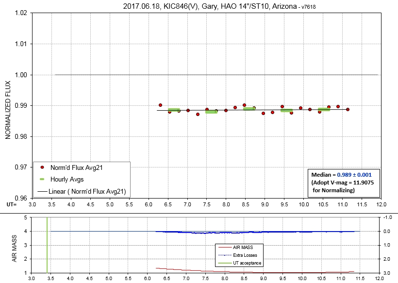
Recovery trend is too slow to be apparent in this 5-hour
observing session.
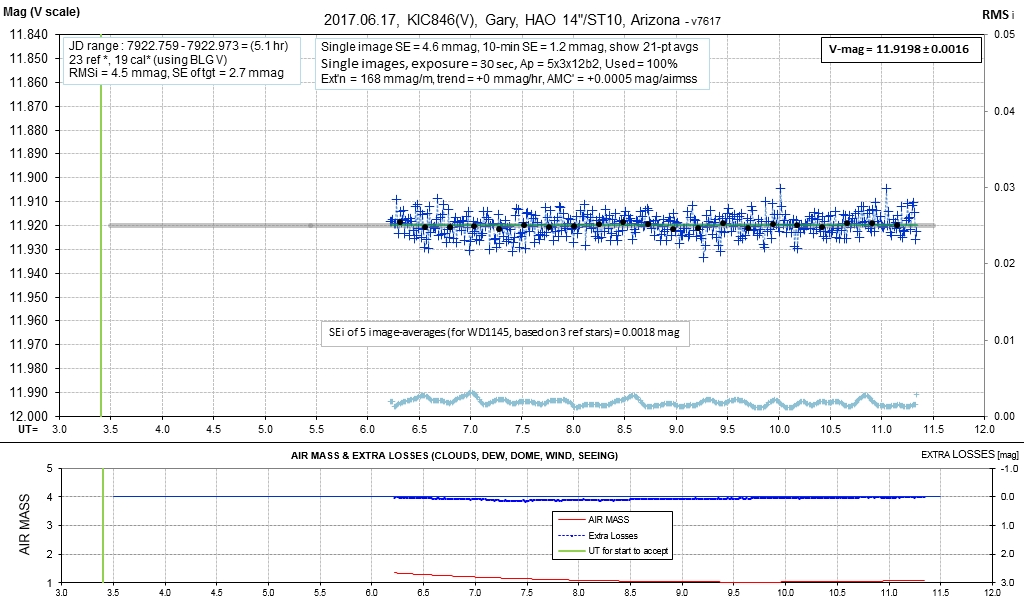
Good observing conditions (no wind, moon far away & faint,
seeing OK).
Good calibration, so overall V_mag will be accurate.
Tutorial on Fading
Star Basics (Reasonable Assumptions and Some Common
Misunderstandings)
Dust Cloud Appeal
Modelers like dust clouds when trying to explain star fadings that
aren't obviously due to binary eclipses or exoplanet transits.
This is because for a given amount of mass small particles can
block more light than a body with the same mass. For example, if a 10 km diameter asteroid is pulverized
to 1 micron radius dust particles it is possible for such a
cloud to obscure (scatter and absorb) 20 % of Tabby Star's
light, whereas the original asteroid would obscure only
0.00000000002 %. This dramatic difference is due to the fact
that the ratio of area cross-section to volume (i.e., mass) is
proportional to 1/size.
Dust Cloud "Optical Thickness"
Dust clouds are almost certainly causing the fades of
Tabby's Star, hereafter abbreviated as TS. That's my position, and
I acknowledge that some reasonable people will want to emphasize
an alternative. If the particles are dispersed enough that most of
them don't overlap along a typical line-of-sight, we say that the
cloud has a small optical depth. This means that some (possibly
most) starlight will penetrate the cloud when the cloud passes in
front of the star. An optically thin cloud can cover the star
completely without producing a large fade. As an alternative, a
dust cloud can be "tightly packed" such that essentially no star
light passes through. That cloud is referred to as "optically
thick." If such a cloud
has a small projected area ("solid angle"), which is much
smaller than the star, it could produce an equally small amount
of fade as it passes in front of the star. Both cloud
types can produce a 1% fade, or a 20% fade, or any fade amount. It
is observationally difficult to distinguish between the two cloud
types (optically thin vs. optically thick). Observations that show
a smaller fade amount at longer wavelengths (e.g., smaller fade at
red vs. blue) would constitute good evidence for an optically thin
cloud with particles having radii of about a micron. However, if
the same size particles are in an optically thick cloud, with
sharp boundaries, then it would produce fade amounts that are the
same at all wavelengths. Large, solid objects will produce the
same fade amount at all wavelengths.
When Kepler measured a dip with depth 20% it could have been
produced by an optically thick dust cloud that covered 20% of the
star's solid angle (projected area), or it could have been
produced by an optically thin cloud that covered the entire star
but had an optical depth of only ~ 0.22 (noting that e-0.22
= 0.80).
IR Excess
The temperature of the dust will depend on
its proximity to the star. If, for example, it's at 1.6 a.u. from
TS (P = 618 days), the dust will be at a temperature of ~ 450 K
(+180 C). Or, consider a dust cloud in a closer orbit, at 0.52
a.u. (P = 114 days); dust could be as hot as ~ 800K. Imagine that
the dust cloud is optically thick (at Near IR wavelengths) and
that it has a projected area 100 times greater than the star's
projected area. The next graph shows a predicted "spectral energy
distribution" for the star, the dust cloud, and star plus dust
cloud.
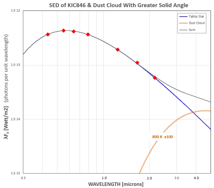
Figure 2.1. Spectral Energy Distribution (SED) of a
hypothetical star and large (optically thick) dust cloud. The red
diamonds are from measured magnitudes of TS, the matching SED is
for Teff = 6400 K (blue trace), and a dust cloud spectrum is shown
for Teff = 800 K and projected area 100 x TS (brown trace). The
gray trace is the sum of both components, and corresponds to
what should be measured for such a hypothetical system.
This graph shows that for a dust cloud to show up in
measurements at IR wavelengths (i.e., called "IR excess") it would
have to: 1) be much larger in projected area than TS, 2) be
optically thick, and 3) be hot (close to TS, orbiting with a short
period). An optically thin cloud would have to be either hotter (in
orbit closer to TS), or larger than the hypothetical model shown in
the figure, for it to produce a meaasureable IR excess. It is
therefore possible for extensive fadings to occur without an IR
excess to be measured. In other words,
the lack of a measured IR excess does not rule-out the
presence of extensive dust clouds.
IR Excess Flux Nonsense: Some comments at
"reddit" (which I rarely view and never contribute to) claim
that if the long-term fade is increasing (and possibly
accelerating), there should be an increase in IR flux. Not
true. As described in my discussion of IR excess below
a dust cloud that's orbiting at a distance of 0.25 a.u.
(with a period of 40 days), will have a temperature of
800 K, and if it is opaque and covers a solid angle 100
times Tabby's Star, it will produce an IR excess that is too
small for detection (as shown by a SED graph, below). If you
relax any of these assumptions (e.g., more distant,
optically thin, < 100 x solid angle of TS), which the
present fade data permit, the IR excess will be even less
detectable. Therefore, the lack of any observed increase in
IR flux (at wavelengths < 5 micron) does not argue
against the presence of a dust cloud that is being
considered for explaining the observed long-term, slow fade.
Distance/Period Relationship
Given that TS has a mass estimated to be 1.43 times solar, we
can relate planetary orbital radius and period using the
following:
a3 = 1.43 × P2
Where "a" is circular orbital radius in astronomical units,
a.u., and P is period in years. This relationship is shown in
the next graph.
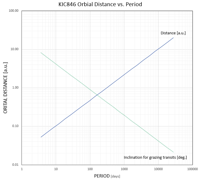
Figure 2.2. Orbit radius vs. period (blue line). The
apparent radius of TS (degrees) as viewed by an object in an
orbit with the x-axis period is also shown (green
dotted line).
Here's an example of how to use the above graph. Suppose we are
considering Kepler dips #5 and #10 to be produced by the
same object. They are separated by ~ 756 days. An object
orbiting with that period would be at 1.9 a.u., and from that
orbital distance TS would appear to have a radius of 0.23
degree. If this object's orbit were inclined with i = 89.77
degree, it would produce a grazing transit as viewed from Earth.
Temperature of Asteroids and Dust vs. Orbital Distance
An object without atmosphere, such as an asteroid, will be
heated by TS to temperatures that depend on whether the object
is rotating slowly (such as synchronously) with a period that is
much shorter than orbital period. For the synchronous case, and
assuming a Bond albedo of 10% (fraction of star radiation that
is reflected), the sub-solar tempearature is given by
Tsurf
(ø) = (579 / sqrt(r) ) * (cos (ø) )1/4
where ø is
starlight incidence angle (zero degrees at sub-solar point) and
r = asteroid/TS distance [a.u.]. The following graph was
calculated from this equation.
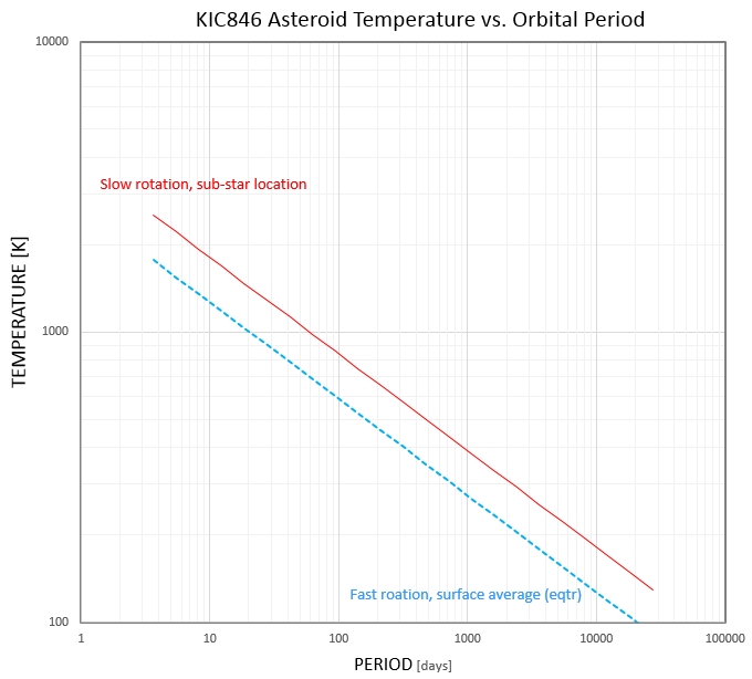
Figure 2.3. Temperature of an airless planetesimal
(asteroid) vs. orbital period (circular orbit). Red trace is
sub-stellar location of a slow-rotating asteroid; blue trace
is an estimate for temperature along equator of a fast
rotating asteroid. Dust could be at temperatures ranging from
the blue dotted trace to above the red solid line trace (as
explained in text).
Using the same example as in the previous section, with P = 756
days, a slow-rotating asteroid will have a sub-stellar
temperature of ~ 430 K. A fast-rotating asteroid will be
somewhat cooler, at ~ 300 K (23 C, or room temperature).
Dust is more complicated, since when a particle is small
compared with the wavelength of thermal emission (a matter of
microns for room temperature dust) the dust has a low
emissivity, and it becomes hotter than nearby large particles. A
calculation has recently been made by Rappaport and van Lieshout
(private communication, 2017), and one aspect of their
calculations is shown in the following graph.
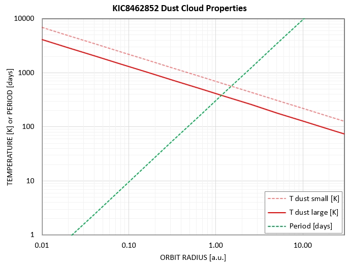
Figure 2.4. Temperature of dust
particles for large radii (> 10 micron, solid red line)
and small radii (< 0.5 micron, dashed red line) versus
(circular) orbital distance from the KIC846 star. Orbital
period is shown (green dashed line). [Based on unpublished
work by Rappaport and van Lieshout, 2017.]
It should be noted that in the above graph there would be no
need to consider the "small particle" temperature result for
distances smaller than about 0.2 a.u., because small particles
at that distance from KIC846 would be so hot that they would
immediately sublimate and disappear. Even the large dust
particles would disappear at distances closer than ~ 0.07 a.u..
Given that Tabby's Team has found evidence for a wavelength
dependence of depth (deeper at short wavelengths) we can assume
that a component of small particles exist. How small? Smaller
than ~ 1 micron. Since these particles will be among the hotter
than larger particles, we may conclude that the dust clouds that
produced the May and June fade features are in orbits farther
from the KIC846 star than ~ 0.2 a.u.. These distances have
corresponding orbit periods of 30 days and longer. Therefore,
any suggestions that the May and June fades will repeat at
intervals shorter than ~ a month will have to confront the
finding of depth dependence upon wavelength.
Importance of Inclination
Inclination of the orbits of the dust clouds is a very important
parameter for deriving a physical model to account for
observations. Inclination was for some silly reason defined to be
90 degrees for an edge-on orbit orientation, and zero degrees when
the orbit is viewed "face-on." An exoplanet won't produce transits
for an inclination of zero degrees, and will always produce
transits when inclination is 90 degrees. For exoplanet transits in
which the entire projected area of the planet passes within the
disk of the star will produce a fractional loss of starlight given
by (Rp/Rs)^2, where Rp is planet radius and Rs is star radius. An
observer outside our solar system, and located in the ecliptic
plane, would see Jupiter transit with depth of 0.4% (0.004
magnitude, or 4 mmag). If the planet, or asteroid, orbits in front
of the star in a way that appears to pass through the star's
central point, we say that the transit path has an "impact
parameter" of zero. If it passes tangent to the star's edge, we
say the transit path has an impact parameter of one. Dust clouds
produced by a solid object, such as an asteroid, will start out with the same orbit as the object, so
such a dust cloud's inclination will be the same as the object's.
The concept of "impact parameter" for a dust cloud loses meaning
the larger it gets. When small, such a cloud's impact parameter
will have to be < 1 in order to produce a fade, but if the
cloud becomes large it can produce a fade even for impact
parameters > 1. Tabby's Star is suggested to have a radius 1.58
x Solar Radius, so Rs = 1.1e6 km for Tabby's Star. An object
orbiting at 1.6 a.u., for example (i.e., 2.4e8 km), will appear to
have a radius of 0.26 degree (same as our sun as viewed from
Earth). For transits of objects at 1.6 a.u. from Tabby's Star to
produce transits the inclination of the object's orbit must be
closer to 90 degrees than 89.75 degree (i.e., i > 89.75). Only
one out of 350 star solar systems will have such a favorable
orientation (producing transits of exoplanets at such an orbital
distance).
A Possible Viewing Geometry
Imagine a situation in which an object is orbiting with a
radial distance from TS of 2.9 A.U.; it will have a period of 1512
days (notice that this is twice 756 days). The star will have an
apparent radius of ~ 0.3 degree as viewed by the object. If the
orbit is inclined 89.7 degree, as viewed from Earth, the object will appear
to pass in front of the star close to an edge of the star (one of
the poles). The next figure is a diagram showing dust clouds
passing over the north pole of TS, moving to the right. Only about
half of the cloud will block starlight during a passage.
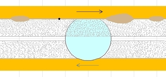
Figure 2.4. As viewed from Earth the projected path of
dust clouds (3 tan blobs) in an orbit inclined 89.7 degree will
pass in front of the "north pole" of TS on the near side of the
star, moving to the right. Nothing is observed when the same
dust clouds orbit on the far side, behind the star (lower
path, moving to left). This geometry is for an orbit distance
from TS = 2.9 a.u., with a period of 1512 days. The dark dot
corresponds to a planet with a radius of 30,000 km, which is
slightly larger than Neptune (or 0.4 x R_Jupiter), and it
produces a dip depth of 0.08 % (0.8 mmag). [This diagram is
borrowed from a modeling exercise for WD1145, which has many
dust clouds orbiting with a period of 4.5 hours. A ring system
is shown that accounts for an IR excess. The dotted region
inside the ring system depicts circumstellar gas that extends in
to within 10 radii of the star. The ring system and
circumstellar gas disk are not present for TS.]
Dip Depth and Planet/Object Size
Figure 2.4 shows a planet slightly larger than Neptune (1.2 x
radius) as a black dot in relation to the disk of TS (1,100,000 km
radius). Such an object would produce a dip depth of 0.08 % (or
0.8 mmag). Since dip depth is proportional to (R_planet/R_star)2,
to achieve a depth of 1%, for example, we require R_planet = 0.1 x
R_star, which is 110,000 km radius (or 1.5 x R_Jupiter). The
following graph shows dip depth vs. planet radius.
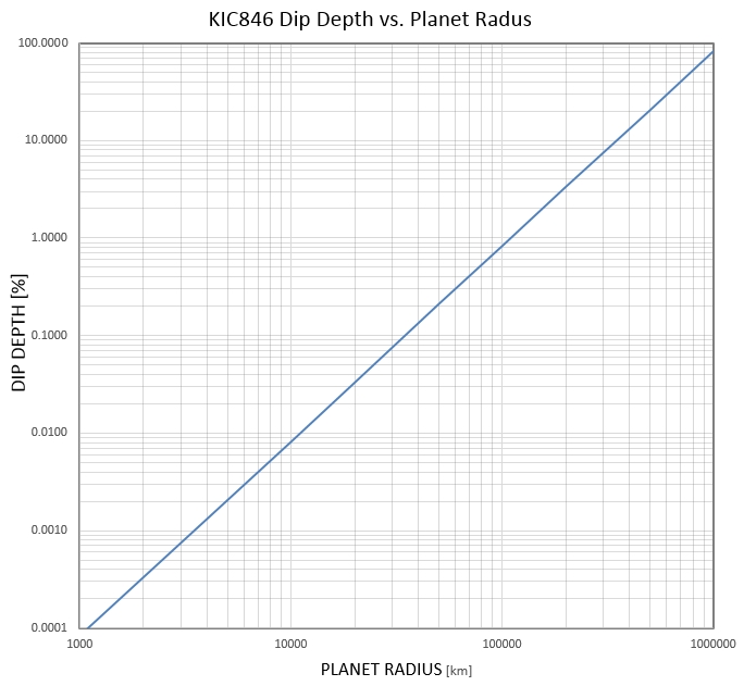
Figure 2.5. Dip depth vs. planet radius (or, optically
thick dust cloud with equivalent circular radius).
The reently measured dip depths of 2% require either a planet size
of 150,000 km radius (2.2 x R_Jupiter), or an optically thick dust
cloud with the same equivalent circular radius. The same depth
could be achieved by a dust cloud that covers the entire star that
has an average optical depth of ~ 0.02.
A Way to Dispell Mega-Structure Speculation
Suppose it is determined that dip depth varies with wavelength.
Dust clouds would provide a ready explanation for such a finding.
In addition, the particle size distribution could be modeled since
the wavelength where fade depth changes occur would indicate the
wavelength where the transition between Mie scattering and
Rayleigh scattering occurs, which in turn would indicate the
typical circumference of the dust.
Mineralogy of the dust particles might also be subject to
constraint, since scattering and absorption, as specified by a
mineral's real and imaginary parts of the dielectric constant,
influence the shape of extinction (scattering plus absorption) vs.
wavelength. Such a modeling effort would require observations of
high quality. The resulting dust cloud model would correspond to
low optical depth with large areal extent.
A structure made of metal would not block light differently at
different wavelengths (assuming the metal is thicker than the
dimension of a few molecules). Therefore, if it is found that dip
depth is less at longer wavelengths (i.e., red and infrared) vs.
shorter ones (blue or green), then this would present a serious
challenge to those who want TS fades to be caused by alien
structures.
A
Plausible Model for Accounting for Brief Fades and an Inverse
Gaussian Model for Long-Term Fading and Recovery
Short
Version: The long-term fade may be produced by a
stretched-out dust cloud in an outer orbit whereas the brief
but deeper dips that have produced the most excitement are
produced by small dust clouds in one or more inner orbits.
The stretching-out of the outer orbit dust cloud is
straightforward, since any expansion of particles (from a
collision) would send some particles in slightly different
orbits, with slightly different periods. If the periods have
a range of 1%, for example, after 100 orbits the dust cloud
would have a torus shape, and it would be capable of
obstructing starlight continuously. As the torus circular
cross-section expands (without changing orbit size), one
edge of the torus would eventually enter our line-of-sight
to the star. This is when we would observe the beginning of
a gradually increasing fade. The torus may expand to
completely obstruct the star, but when that happens it could
be optically thin and produce only a small fade. Continued
expansion could be accompanied by diminished loss of dust
density along our line-of-sight, so expansion should
eventually be associated with a recovery of star brightness.
The “inverse Gaussian” model that I have employed for
fitting the out-of-transit observations calls for a maximum
fade amount of ~ 3 % in one or two years, followed by a slow
recovery to normal star brightness in 5 or 10 years. During
all of that time there will probably be short fades, lasting
a few days, produced by dust clouds in orbits much closer to
the star (but not closer than ~ 0.2 a.u.), with orbit
periods of at least 4 weeks (but not less, due to the
temperatures for closer orbits causing the particles to
sublimate to gas).
Assume that the KIC846 system has recently undergone
collisions, possibly related to a passing star disrupting the
"Oort" cloud of planetesimals (objects of all sizes), some of
which would have changed orbit eccentricity causing them to enter
the inner solar system. Suppose further that collisions occurred
with existing planets in the inner solar system, orbiting at 0.2
and 2.0 a.u.. The resulting debris would produce clouds orbiting
with periods of 30 days and 900 days. The temperature of the dust
will range from 750 K to 1300 K (for the inner orbit) and 300 to
500 K (for the outer orbit). [These temperature calculations are
based on unpublished work by S. Rappaport and R. van Lieshout,
private communication, and soon to be submitted for publication in
MNRAS by S. Xu et al. As an aside, these calculations can be
viewed as ruling out smaller orbits, with shorter periods, for
causing the brief fade events first discovered by the Kepler
K2 mission, and recently documented and given names Elsie and
Celeste. I won't explain more until the aforementioned articles
are in the public domain.]
The planets are in orbits that are viewed almost edge-on, inclined
to our line-of-sight by a small angle, such as 1.0 degree (i.e.,
inclination = 89 degrees). We must associate the inner orbit
collision (and the fragments created) with brief fade events, and
we must associate the big outer orbit collision (and those
fragments) with the slowly developing long-term fade of
out-of-transit (OOT) brightness. Notice that for an inclination of
89 degrees the distance between our line-of-sight and the two
orbits are 0.0035 and 0.035 a.u., respectively (orbit radius x sin
(90 - i)). These are the distances that an expanding dust cloud
will have to achieve in order to block starlight from our view. If
the dust cloud expansion velocities were the same (just a starting
guess) then the outer cloud would take 10 times longer after a
collision to begin blocking starlight. During that time it will
have been sheared to all longitudes of the orbit. The dust cloud
would soon take on the shape of a torus, with a constant average
orbit radius but with an expanding cross-section. In other words,
blockage of starlight by the outer cloud will not vary on
timescales much shorter than the 900-day orbit. All of those torus
blockages of starlight could have been set in motion by one big
collision (with a planet at 2.0 a.u.).
The inner cloud, however, will be more changeable for two reasons:
1) the interval between a collision fragment's production of dust
and the time it reaches our line-of-sight to begin blocking
starlight is much shorter (1/10 of that for the outer orbit,
assuming similar isotropic velocities), and 2) the dust
temperatures for the inner dust cloud can be hot enough that small
particles will sublimate and become a gas that doesn't block
starlight (except at very specific and narrow wavelengths). This
last point means that the inner dust clouds can come into
existence and then disappear (due to sublimation) on short
timescales, possibly comparable to their orbit period of 30 days.
Notice that I referred to "fragments" from an inner orbit
collision as sources for the dust clouds. I am suggesting that the
brief but deep fade events are caused by fragments from possibly
one collision with a planet in an inner orbit (0.2 a.u.). These
fragments will have periods similar to the planet from which they
were broken off, and they will be the source for dust clouds
producing fade events.
The other collision, with a planet in the outer orbit (2 a.u.),
would not have to occur at the same time as the inner orbit
collision. The outer orbit collision could have occurred centuries
ago. In fact, it probably had to have occurred at least a century
ago in order for the dust from the collision to become
stretched-out into torus shape, and for the torus cross-section to
have expanded enough to enter our line-of-sight to the star and
begin a long-term fade.
Consider again the expanding torus of dust in an outer orbit. It
will begin to produce a fading that starts long after the original
collision (given by orbit
radius x sin (90 - i) / dust ejection speed). As the
cross-section of the torus continues to expand it will become less
dense along our line-of-sight, and thus begin to block less
starlight. The amount of fade by this long-term component will be
determined by the line-of-sight column content of dust (and
involving a size distribution spectrum).
The above physical model has features that are compatible with
observations of both the brief fades, lasting a few days and
capable of being deep, as well as a decoupled long-term fade that
is gradual in its rise for blocking starlight and gradual in its
recovery to negligible blockage, with characteristic timescales of
years. [For an extensive discussion of
fragment-produced dust clouds that produce fade events
orbiting a white dwarf, WD1145, read https://arxiv.org/abs/1608.00026
]

Comparing Kepler
with Recent Light Curves
Here's the last 140 days of the Kepler light curve. It
shows the deepest dip observed, 21%, Dip #8 at Kepler Day 1520
(abbreviated as d1520). The second deepest dip, Dip #10 with depth =8% is at d1568.
The dip at d1540 (Dip #9) has generated interest due to its
symmetric pattern of a 3%
dip flanked by 1.1% dips on either side, separated from the main
dip by ~ 3 days. Many people have been attracted to the idea
that Dip#9 is produced by a large planet with rings, and it's
the rings that produce the two flanking dips.
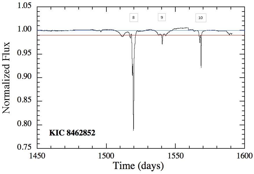
Figure 3.1. Kepler light curve for the
last 140 days of TS observations.
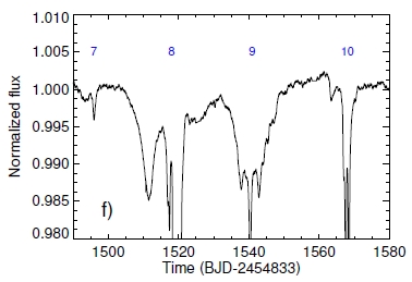
Figure 3.2. Same
data on expanded date and normaled flux scales.
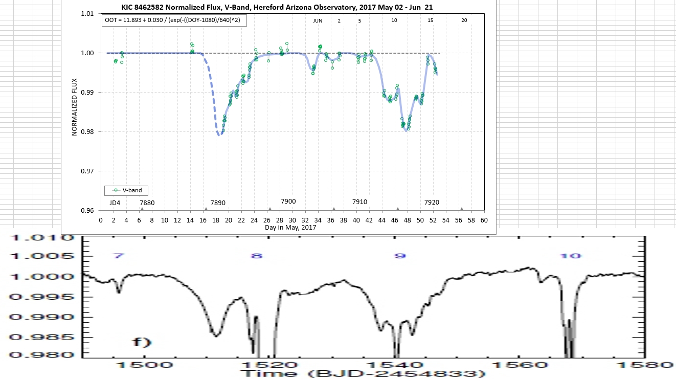
Figure 3.3. Comparison
of Kepler and Gary light curves using similar date and
normalized flux scales. [The observations panel is not
up-to-date; I'm not a believer in this association so my
motivation to update is low.]
The similarity of structure for the Kepler Dip #9 and the
recently-measured Jun 16 dip is apparent. Even an earlier dip
(before Kepler Dip#8) has a correspondence with the May 19 dip.
Only the Kepler d1520 feature (21% depth) is missing in recent
data (maybe it's a dust cloud in a different orbit than the Kepler
d1512 and d1540 features). I'm not bothered by the difference in
depth of the Kepler d1540 dip (3% vs. 2%) because dust clouds
should disperse over time, and produce smaller dips. This is an
interesting similarity of pattern (but I'm not a "believer"!
Long Term Trends
My original purpose for starting KIC846 observations 1.7 years ago
was to measure long term trends; catching fade events wasn't my
goal. I think I've measured a long term fading trend, and it seems
to be "accelerating."
If dip measurements are excluded from consideration there are
long-term trends in TS "out-of-transit" brightness. Here's a plot
of my V-mags during the past year. Note the slight curvature for
the model fit.
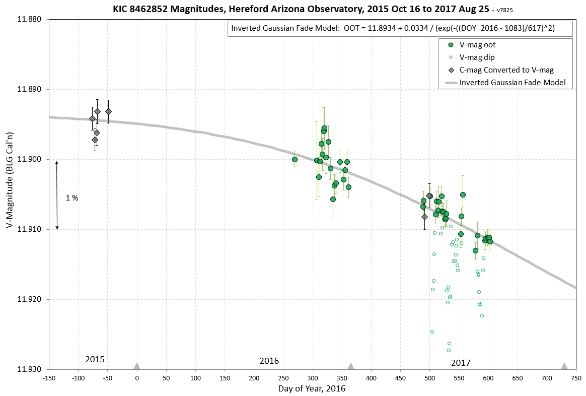
Figure 4.1. V-mag's for TS during the past 300 days. Filled
circle symbols are judged to be "out-of-transit," or made when
dips were not underway. Open circle symbols are the dip
data. The late 2016 data exhibits a 29-day periodicity.
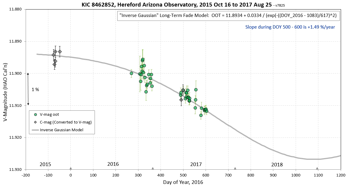
Figure 4.3. A 1.7 year's worth of V filter and
clear filter measurements has been fitted with a model. Only OOT
data are shown. The clear filter magnitudes were adjusted to
match near-simultaneous V-mag measurements. A Gaussian model was
fitted to both sets of measurements. This speculative model
"predicts" a return to "normal brightness" after several years
(after 2021).
The Gaussian model is meant to represent a dispersal of dust from
a giant collision that produced dust that is slowly being spread
out along the orbit where the collision occurred. The dust would
initially produce brief and possibly deep dips, but as it
disperses the dust will be present at all parts of its orbit and
cause a fade that persists for as long as the dust is present in
the orbit plane where it can intercept our line-of-site to TS.
This is just a speculation; I have no idea if this is correct.
A Prediction
I predict that in a matter of months the brightness of KIC846 will NOT plummet to zero, but
the level of interest in KIC846 by the general public will!
This will happen when the professional astronomers present
evidence that the fading events are produced by dust clouds, not
alien mega-structures. The hit rate for my KIC846 web pages, which
is currently about once a minute, will return to the once a month
level, just as they were for the 1.5 years before May 19 of this
year.
I have experience with the fickleness of such things based on my
2013 observations of Comet ISON - that so-called "Comet of the
Century." NASA bought into that terminology, possibly because it
garnered public interest in a project that NASA had funded. I was
the first to dampen enthusiasm when I made the first "recovery"
observation after a 2.5-month hiatus of imaging (due to the sun
being close to the line of sight) as the comet was making its
approach, and I stated that the comet was about a magnitude
fainter than models were predicting, and it might disappoint
during the rest of it's approach to perihelion. NASA continued to
hype the comet, and I attracted a fan club of cynics who trusted
my assessments and almost daily updates more than those by the
professionals. Some unscrupulous web hucksters took pictures from
my web site for posting on theirs with hyper-hysteric
interpretations; one posted a picture I had enhanced to show a
forward jet and on his web site he claimed to show a UFO flying in
formation ahead of the comet. As perihelion grew closer, and the
comet's brightness fluctuated at below expectations, and as my web
page hits grew to ever higher levels, and as experts were quoting
my kill-joy assessments, Discovery Channel scheduled an interview
with me at my observatory to coincide with perihelion passage. But
as the sun's heat sublimated the comet to nothing during closest
approach; public interest immediately plummeted to zero and the
the Discovery Channel interview was canceled. My web page hits
went to nothing, and my life returned to normal. But I was wiser,
for I finally understood the fickleness of public interest in
things scientific.
I predict that by the end September, when the evidence for dust
clouds and prosaic decadal variations are accepted, KIC846 will
join the "Hype of the Century Club" for being "the alien
mega-structure that wasn't."
References
Simon, Joshua D., Benjamen J. Shappee and 6
others, "Where is the Flux Going? The Long-Term Photometric
Variability of Boyajian's Star," arXiv:1708.07822
Meng, Huan Y. A., G. Rieke and 12 others
(including Boyajian), "Extinction and the Dimming of KIC 8462852,"
arXiv: 1708.07556
Sucerquita, M., Alvarado-Montes, J.A. and two
others, "Anomalous Lightcurves of Young Tilted Exorings," arXiv: 1708.04600
Also, see New Scientist link
and Universe Today link.
Rappaport, S., A. Vanderburg and 9 others,
"Likely Transiting Exocomets Detected by Kepler," arXiv:
1708.06069
Boyajian et al, 2015, MNRAS, "Planet Hunters
X. KIC 8462852 - Where's the flux?" link
Ballesteros, F. J., P. Arnalte-Mur, A.
Fernandez-Soto and V. J. Martinez, 2017, "KIC8462852: Will the
Trojans Return in 2011?", arXiv
Washington Post article, 2015.10.15: link
AAVSO Campaign
Notice requesting KIC646 observations
AAVSO LC Generator https://www.aavso.org/data/lcg
(enter KIC 8462852)
Web page tutorial: Tips for amateurs observating faint asteroids
(useful for any photometry observing)
Book: Exoplanet Observing for Amateurs,
Gary (2014): link
(useful for any photometry observing)
My web pages master list, resume
 B L G a r y at u m i c h dot e d u
Hereford Arizona
Observatory resume
B L G a r y at u m i c h dot e d u
Hereford Arizona
Observatory resume
This site opened: 2017.06.18. Nothing on this web page is copyrighted.