This web page intends to show what WD1145 photometric variations may be like during the 2023 observing season. This assumes that similar activity levels exhibit similar photometric behavior. Some of the analysis presented here is a repeat of what was reported by Vandenburg et al. (2015) and Croll et al. (2015), but this analysis leads to some additional "takeaway lessons" that were not reported by the earlier investigators. This work is important for understanding the "activity" plots for the past 9 years.

Average Light Curve During K2 80-Day Observations

The Kepler K2 data for WD1145 consist of 1642 measurements with a cadence of 29.376 minutes. A LC for all data is shown below.

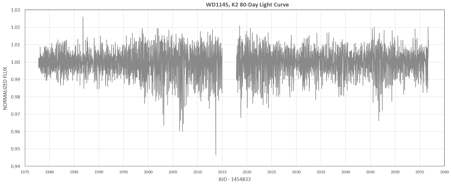
Figure 1. Kepler LC for the entire 80-days of WD1145 observations.

Some of the variation of maximum depth is due to the phasing-up of two or more dips having different periods. Another component is the actual change of depth for the A- or B-system dips (the two most important sources for dip behavior). 

Here's a zoom-in to show a typical 1-day span of data:

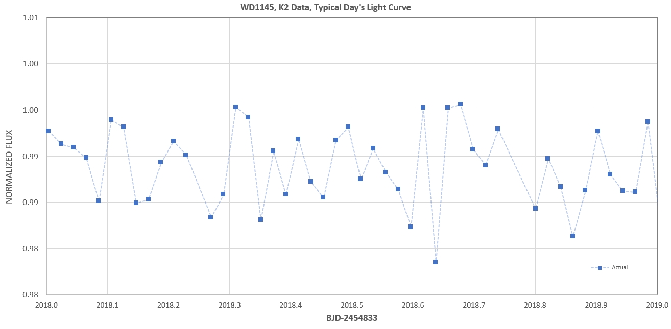
Figure 2. Kepler LC for a 1-day interval, chosen at random.

The variations in the above figure are real; the appearance of being noisy is due to the observing cadence not being shorter than the timescale for actual changes.

Here's a periodogram for the entire data set:

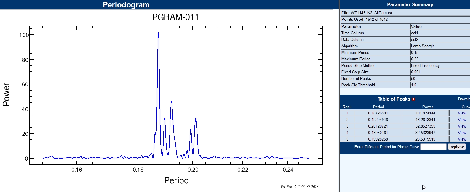
Figure 3. Lomb-Scargle periodogram for the entire set of K2 data, showing at least 5 significant signals.

The following set of 6 figures show my model fitting solutions for the 6 most significant periodicities (exact P values are solved for in each case):

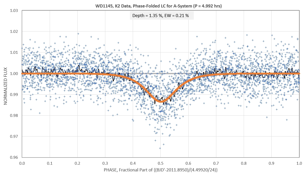
Figure 4. A-system phase-folded LC for the solved-for parameters for the AHS (asymtotic-hypersecant) model (period, phase, depth, width-preceding and width-following).


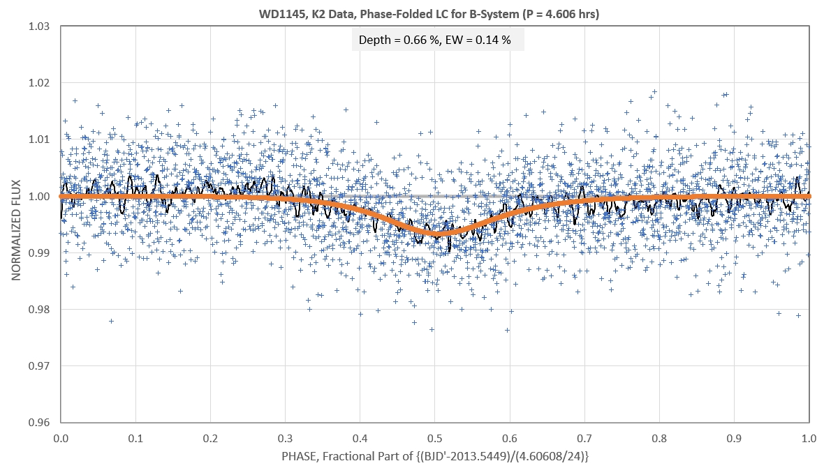
Figure 5. B-system phase-folded LC.


Figure 6. C-system phase-folded LC.


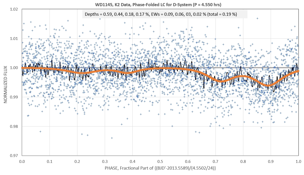
Figure 7. D-system phase-folded LC.


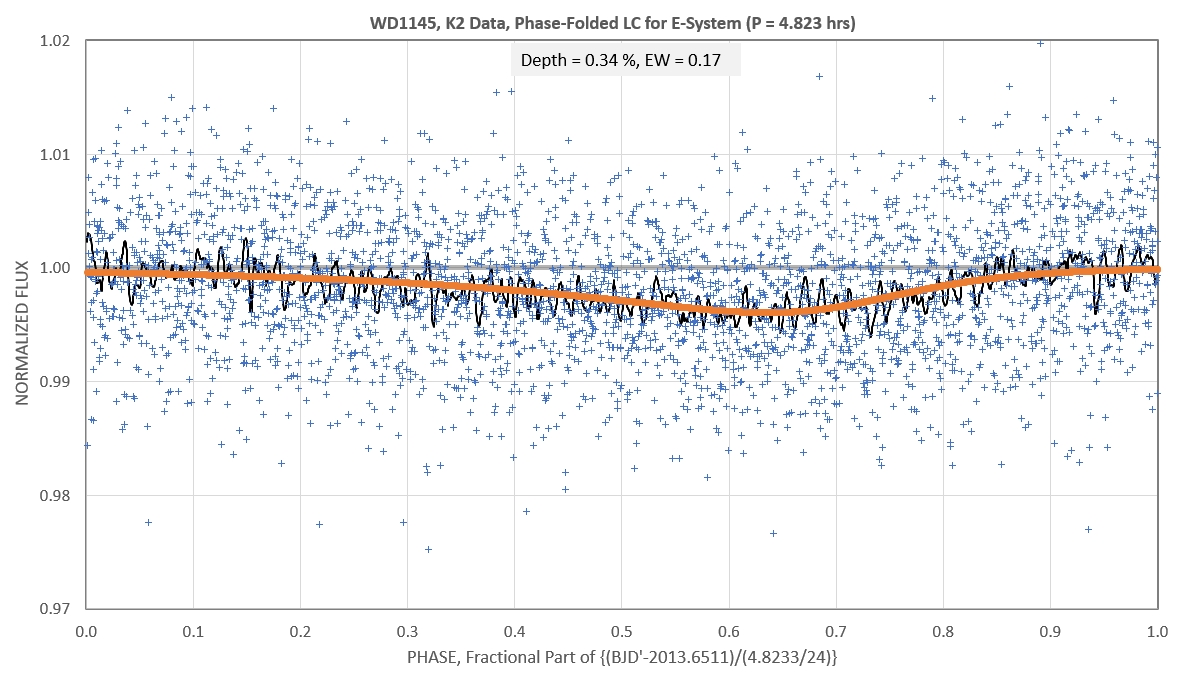
Figure 8. E-system phase-folded LC.


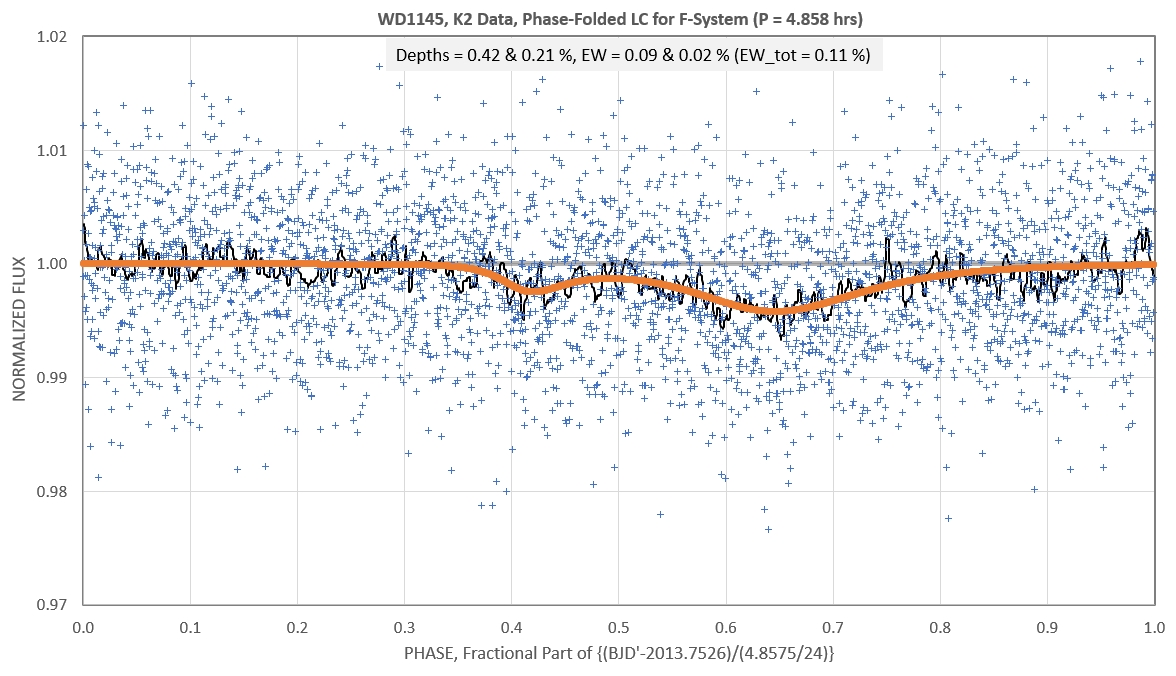
Figure 9. F-system phase-folded LC.

Keep in mind that the above phase-folded LCs and AHS model solutions are for the entire 80 days of K2 data. Actual changes may occur on timescales of days.

How well can the AHS model fit any specific portion of the 80-day data set? Let's apply the model to that 1-day example shown in Fig. 2.


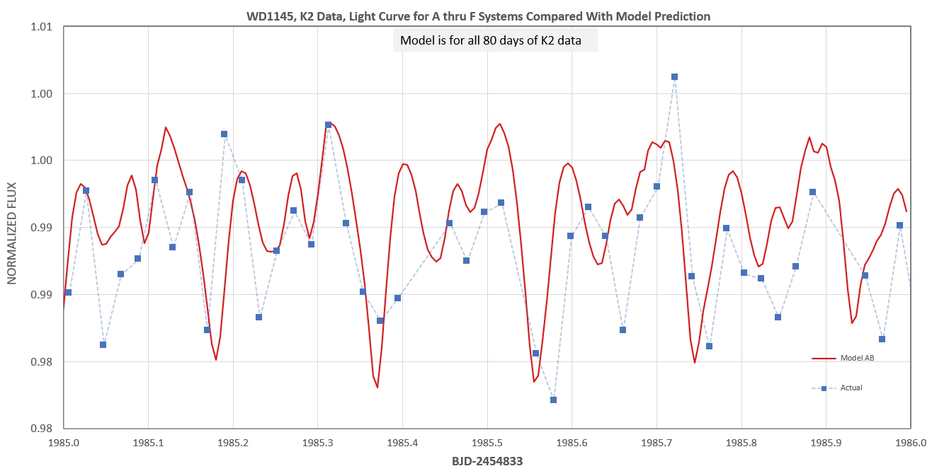
Figure 10. AHS model for the entire set of data applied to one day of data chosen at random.

How did the most active dip evolve during the 11 weeks of K2 observations?


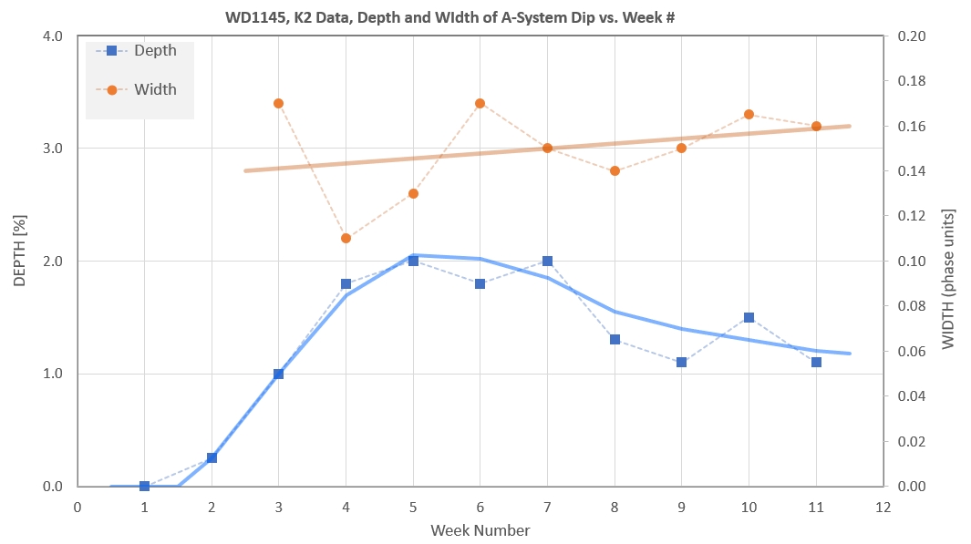
Figure 11. System-A dip appeared during week #2 and exhibited a peak depth 4 weeks later, followed by a slow decline. Dip width remained essentially constant.

Keep in mind that when ground-based observations began (about 7 months after the end of K2) all dips (presumably from the A-system) had widths of ~ 0.04 phase units (10 minutes).

Here's how B-system evolved during the K2 interval:


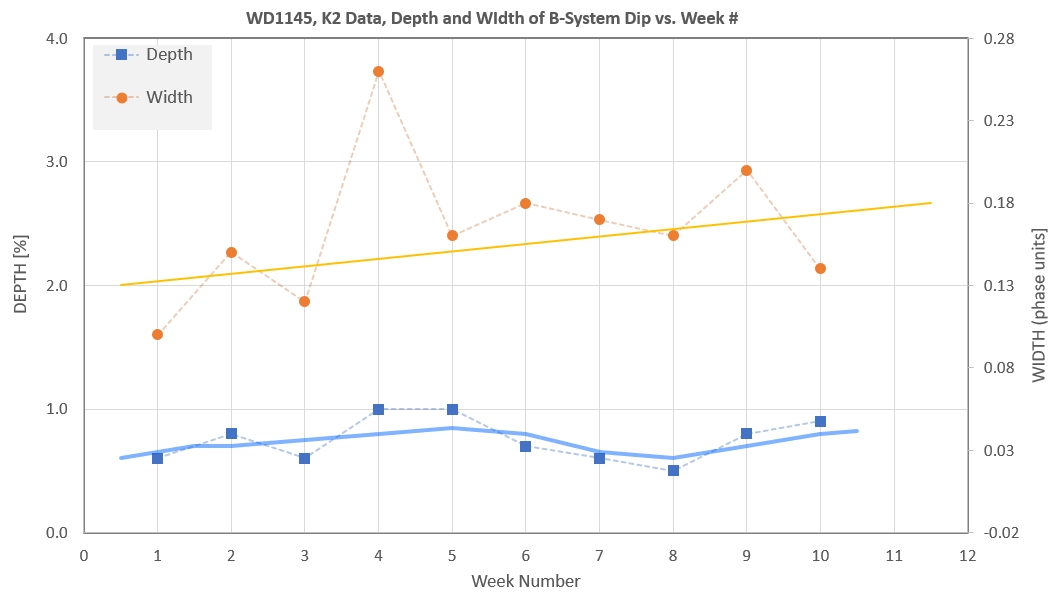
Figure 12. System-B didni't change much during the K2 observing interval. .

Takeaway Lessons From K2 Data

Whereas K2 dips were mostly broad and shallow, post-K2 dips were narrow and deep. The ratio of width is ~ 4 (for both A- and B-systems) and the ratio of depths varied a lot but were as high as 30 (for the A-system). At the present time, in 2023, I think dip widths remain narrow and depths are comparable to K2. In other words, K2 data doesn't include any short-duration dips (that I've noticed), whereas all post K2 dips, when activity level is high, are short duration and usually deeper.

In Fig. 10 there is some correlation of measured and modeled; the amount of disagreement must be due to actual changes on weekly timescales being compared with a model based on data lasting 11 weeks. One possibility is that on weekly timescales the dips are briefer and deeper, and from week-to-week they simply move in phase orbit position in a way that over long tmescales makes them appear to be broader. I've investigated this and the week timescale dips are just as broad as the 80-day breadths. However, the weekly-timescale dips vary in depth significantly. (Somebody should try to eplain sy breadth doesn't change, but depth does - during the phase of low activity level.)

Notice in Fig. 10 that the OOT level is reached a very small fraction of the time. A ground-based observing session will typically be 6 to 9 hours long (~ 0.31 day). For the Fig. 10 example OOT is observed only once or twice per observing session (noting red trace), and it will last only a  few minutes. This should be the situation when most of the 6 periodicities have comparable depths. During the K2 observations the activity level is what can be described as "quiescent." It is tempting to believe that whenever WD1145 is at a similar level of activity the depths for each periodicity will be comparable to what was observed during K2, and the fraction of time for OOT will be low.

When calculating "activity level," defined as the percentage loss of star brightness averaged of many orbits (i.e., long-term brightness loss), the losses for each periodicity should be added. Thus, the loss due to the A-system dip over the a system period should be added to the loss produced by the B-system dip during the B-system period, etc. When this is done for the K2 data a total loss for the 6 periodicities is 1.14 %. Note that the loss due only to the A-system is a mere 0.21 %.

When depths for two (or more) periodicities are comparable there are times when both (or more) dips occur at the same time. This accounts for the deepest dip versus date varying greatly, as seen in Fig. 1.

During 2015 the A-system became extremely active while the other systems remained at a low activity level. The way to show this increase is to plot the A-system activity level for all dates, before and after the 2015 event. This is done in the next figure. 

 
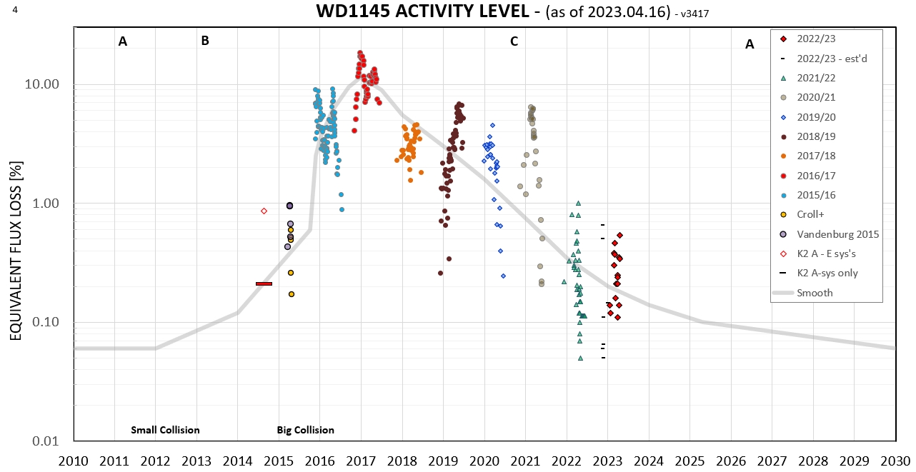
Figure 12. Activity level vs. date. The K2 activity has two symbols in this plot: one is for the A-system (lower bar) and the other is for all periodicities (open diamond). The smoothed trace goes through the A-system activity level symbol.

On a few occasions a dip (or set of dips) appeared after 2015 that belonged to the B-system, but their contribution to overall activity level was small. This figure should therefore be interpreted as "activity level for the A-system.

Since we are now (2023) in a state of low activity level, similar to that for K2, we should be prepared to observe behavior similar to that observed by Kepler. In other words, we should now be observing activity at the 0.2 % to 1.4 % level, with dips having a range of periodicities from 4.49 to 4.86 hours. Observing sessions should therefore be limited to 2 or 3 nights. During one observing session the A- and E-system dips, for example, will experience a phase difference of 0.14 phase units, and during two 2 nights the spread in phase between the A- and E-systems will be 0.89 phase units. So far we're unable to measure depths as low as 1.4 %, the deepest dip during K2, averaged over 80 days. For K2 dips from different systems (periods) they will occasionally add to produce 2 to 4 % depths (see Fig. 1), so it's possible the Gary-Kaye-Mullen observing triumvirate could detect a K2-like activity level.

The picture that emerges from all of the K2 and subsequent ground-based findings is that there are 6 rings with at least one planetesimal and maybe hundreds of fragments in each ring, and they usually don't influence each other. For example, in 2015 something happened in the A-system ring that increased its dust production activity dramatically (almost 100-fold), and the other rings remained relatively inactive. If the abrupt rise in A-system activity was due to a collision in the A ring, then debris was mostly confined to the A ring. The fact that dips, both during K2 and post-K2, endure for weeks, at least, means that a steady-state rate for dust production has to match the steady-state rate for dust loss (due mostly, I suspect, to Keplerian orbit shear).

Return to the calling web site: http://www.brucegary.net/zombie10/