Introduction

The goal for light curve photometry is to have measured magnitudes adhere as closely as possible to the correct light curve variation. Given that we usually don't know all aspects of the correct LC variation a priori, the next best thing is to have measurements adhere as closely aqs possible to a best fit LC that's compatible with a priori knowledge. Normally, the a priori knowledge includes the assumption that the OOT portions of the LC should be a smoothly varying function that can be fit by only a temporal trend and air mass curvature components. Another example of a priori knowldges is that ingress and egress should be the same length, and other respects the LC should be symmetric about the mid-transit time. These simple assumptions allow any specific set of LC measurements to be evaluated in terms of "model-referenced RMSi," which I'll define as the RMS of individual (image) measured magnitudes with respect to a best fitting model. If the model is capable of representing the actual LC variation then "model-referenced RMSi" should be the same as RMSi, provided systematic errors are small, where RMSi is the RMS of individual (image) magnitudes based on short-term scatter. When systematic errors are present they will usually vary on timescales longer than the interval between measurements. Thus, systematic errors will cause "model-referenced RMSi" to be larger than "RMSi." One goal for the serious observer should be to evaluate the magnitude of systematic errors by comparing "model-referenced RMSi" with "RMSi," which can be done by orthogonally subtracting the first from the latter.

RMSi, or short-term scatter, is influenced by three principal components: 1) thermal noise from the CCD chip and readout electronics, 2) Poisson noise, and 3) scintillation. The remainder of this web page is devoted to estimating RMSi based on the way these three sources depend on telescope aperture, air mass, reference star choices and photometry aperture size.

Deriving RMSi

My preferred way to determine RMSi is to compare each individual measurement with the median of it neighbors, where approximately 6 neighbor measurements are used. The number of neighbor readings could be 3, 6, 8, etc, and each choice has an associated correction due to the fact that the median of a finite number of measurements will itself have an uncertainty. Using "median" instead of "avearage" reduces the influence of outliers on the resulant RMSi. If 6 neighbor values were averaged the average would exhibit an uncertainty of 1/sqrt(5) of the RMSi. Since I'm using medians we have to add an extra 15%. thus, with 6 neighbors median combined the median will exhibit an SE of 1.15/sqrt(5), which is 0.51 * RMSi. When a value is compared with this neighbor median the difference will exhibit an SE of sqrt(1 + 0.51^2) = 1.12 * RMSi. Therefore, when viewing a set of differences of values from the median of 6 neighbors we should assume that their RMS is actually 1.12 times the RMSi that we're trying to evaluate. 

Predicting RMSi Thermal

After calibrating an image (bias, dark and flat), and before any star alignment adjustments are made, the individual pixels will exhibit an RMS variation in areas free of stars that I will call "pixel noise," Ni. For my CCD, an SBIG ST-8XE, Ni = 7.5 counts when the CCD is cooled to about -25 C. Propogating errors for summing counts within a signal aperture, and subtracting an expected level from a sky background annulus, and converting to mmag yields the following simplre result (as explained on pages 128-129 of my book, Exoplanet Observing for Amateurs, Second Edition):

    SE(thermal) [mmag] = 1086 × sqrt(s) × Ni / Star Flux [counts]                                                                                                                  Eqn 1

Each reference star is subject to an uncertainty given by the same equation (but with different star flux values), and when several reference stars are averaged their ensemble SE is given by:

    Ensemble SE for reference stars = {sqrt (SE₁² + SE₂² + SE₃² + … +SE_n²)} / n, where SE_n is SE for reference star n.                              Eqn 2

This is a general equation that applies to all three sources of noise (thermal, Poisson and scintillation) when ensemble photometry is employed. Our goal for this section is to calculate “ensemble SE for target” for the thermal component, and this is done by orthogonally adding SE(target) and the above “ensemble SE for reference stars” for the thermal cources. Every star field is different, so tere is no simple way to calculate the way all these errors propogate to a final SE(thermal) value excpet in a computer program or spreadsheet that takes into account the star fluxes for all stars, the signal aperture used and the Ni value for the observing session under consideration. I have implemented these calculations in a spreadsheet used to process CSV-files imported from MaxIm DL's photometry solutions. In order to illustrate some concepts it will be instructive to consider a couple cases.

Consider a "standard case" in which the target star has a peak flux of 30,000 counts (~ halfway to saturation), the PSF is a Gaussian shape with FWHM = 4.0 pixels, and one other reference star is used that is 0.3 magnitudes fainter (75% the flux). The target and reference stars will have a flux of 685,300 and 514,000 counts. Next, assume that these stars are measured using a photometry circle with radius of 10 pixels, and assume Ni = 7.5 counts. SE(thermal) = 1086 × sqrt(314) × 7.5 / (685,300 & 514,000) = 0.21 & 0.28 mmag. After subtracting the target's magnitude from the reference star's magnitude, SE(thermal) = 0.35 mmag. When the target star is the brightest star in the FOV, even the use of many reference stars can exceed by a large amount the target star's SE, so the "standard case" just considered is close to ideal. For the case for HAT-P-13, for example, there is a nearby reference star that is 0.3 magnitude fainter than HAT-P-13 (that's why I chose hthis example).

Predicting RMSi Poisson

The Poisson noise component is slightly easier to caluclate. We need to assume a value for CCD "gain," which relates the total counts from a star to the number of photons that released photoelectrons to produce that count. Typicaly, it takes ~ 2.5 photons to produce one count. So when the total counts from a star is 685,300 there must have been ~ 1.7 million photon abasorption events leading to that count. Poisson theory states that when this number is large (and 1.7 million is large enough for this to apply), SE = sqrt(Number). So the SE on 1.7 million is 1309 events, or converting to counts we have an SE of 524 counts. Converting to mmag units, SE = 1086 * 524 / 685300 = 0.83 mmag. The equation tha bypasses intermediate steps is

    Poisson Noise SE [mmag] = 1086 / sqrt (CCDgain × StarFlux[counts])                                                                                                    Eqn 3

If a reference star is used that's 0.3 mag fainter, it will also have a Poisson SE of 0.96 mmag. After subtracting the target star's magnitude from the reference star's magnitude we will have a Poisson SE of 1.27 mmag.

Predicting RMSi Scintillation

Scintillation is determined by telescope aperture, air mass and exposure time according to the following famous equation ((Dravins et al, 1998): 

Let's ignore the observing site altitude term, exp(-h/ho, by assuming an altitude of 4700 feet for all calculations (my site's altitude). The equation then becomes  

    Scintillation [mmag] = 5.35 × (14 inches / D)^2/3 ×AirMass^1.75 / sqrt(g[sec])                                                                                            Eqn 4 

where D is telescope aperture [inches]and g is exposure time [seconds]. If the above star flux counts are obtained using a 14-inch telescope from exposures lasting 60 seconds, then SE(scint) = 0.69 mmag at zenith, and higher values at lower elevations. All stars in the FOV will exhibit uncorrelated fluctuations of this level, so when a target star is compared with one reference star, regardless of the reference star's brightness the component of scintillation noise will be 0.98 mmag for the situation under consideration. 

Predicting RMSi for various telescope configurations

The previous three sections provide a means for calculating what to expect using various telecope apertures and air mass values for a specific target. These calculations will be for the situation of observing HAT-P-13 and using one reference star that is almost as bright as the target. Here's the star field with target "h13" and a nearby reference star identified.

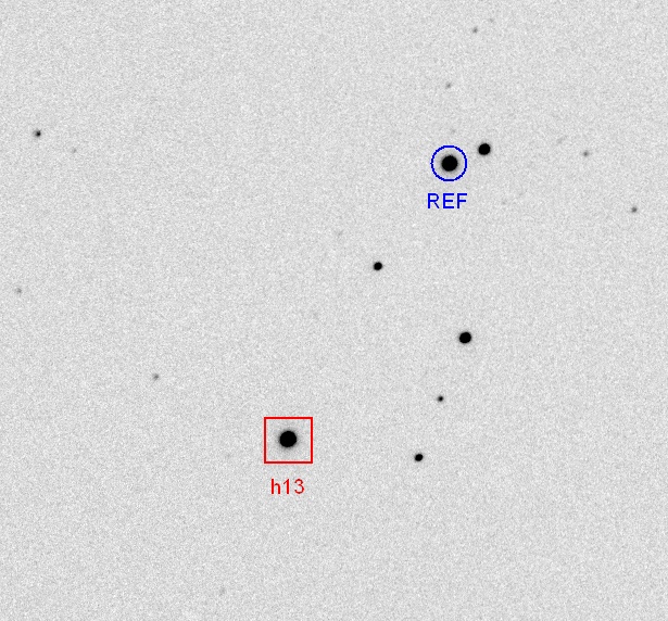
Figure 1. FOV 8.8 x 8.2 'arc, north up, east left, showing HAT-P-13 (labeled "h13") and a nearby star that will be used as reference for the case study of this web page. FWHM = 3.9 pixels. A Celestron 11-inch and CBB-filter were used.

In this image a 11-inch telescope was used with a CBB-filter for a 15-second exposure. The star fluxes are 160,000 counts for h13 and 121,000 counts for the reference star. For h13 the maximum count, Cmax, was 7508. The air mass was 1.14, CCD gain was 2.5 electrons/count, and Ni = 7.5 counts. I will assume 60-second exposures for calculating RMS values. For 60-second exposures we can expect Cmax for h13 = 30,000 counts, which is close to optimum for LC observing (as seeing varies Cmax will vary inversely with the square of FWHM, so we need about this much safety margin to be sure Cmax doesn't exceed the CCD's linearity limit, which is ~ 52,000 counts for my CCD). For g = 60 seconds, the star fluxes will be 640,000 and 484,000 counts.

We calculate SE(thermal) by referring back to Eqn 1, SE Thermal [mmag] = 1086 × sqrt(s) × Ni / Star Flux [counts]. SE(thermal) = 0.23 mmag for h13 and 0.30 mmag for the reference star. After comparing h13 with the reference, we can predict SE(thermal) = 0.38 mmag.

We calculate SE(Poisson) by referring to Eqn 3, SE Poisson [mmag] = 1086 / sqrt (CCDgain × StarFlux[counts]). SE(Poisson) = 0.86 and 0.99 mmag. After comparing h13 with reference we get SE(Poisson) = 1.31 mmag.

We calculate SE(scint) by referring to Eqn 4, SE Scintillation [mmag] = 5.35 × (14 inches / D)^2/3 ×AirMass^1.75 / sqrt(g[sec]). For D = 11 inches, and air mass = 1.17, SE(scint) = 1.07 mmag for both stars. After comparing h13 with reference, we get SE(scint) = 1.51 mmag.

The orthogonal sum of all three noise sources is RMSi = 2.03 mmag. This RMSi will serve as a reference for other values calculated for other telescope apertures and air masses.

RMSi doesn't have a penalty for poor duty cycle. For example, a large aperture telescope might produce very low RMSi values but if most of an observing session is spent downloading images the amount of information obtained per unit of observing time could be low. Let's define something called "predicted RMSi per 10-minutes of observing time." This will be a more useful parameter for considering alternative observing strategies. I shall assume that each image has a download and settle time overhead of 10 seconds. In the following analysis I will calculate exposure time that leads to Cmax = 30,000 counts, assuming FWHM = 4 pixels. I will also prevent exposure times from extending beyond 60 seconds because longer exposure times run the risk of producing a too high incidence of outlier rejections (e.g., spoiled images due to cosmic rays, poor seeing, airplane of satellite tracks, etc).

Here is a plot showing the breadown of the three components of noise for a 11-inch telescope versus air mass.

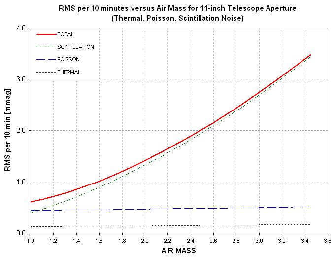
Figure 2. "10-minute RMS" for the three noise sources versus air mass for a 11-inch telescope, with duty cycle taken into account.

This plot shows that near zenith Poisson and scintillation noise are comparable (for an 11-inch telescope). However, beyond air mass ~ 1.5 scintillation dominates. Thermal noise is never dominant.

The next plot shows total RMS noise per 10 minutes for a selection of telescope apertures.

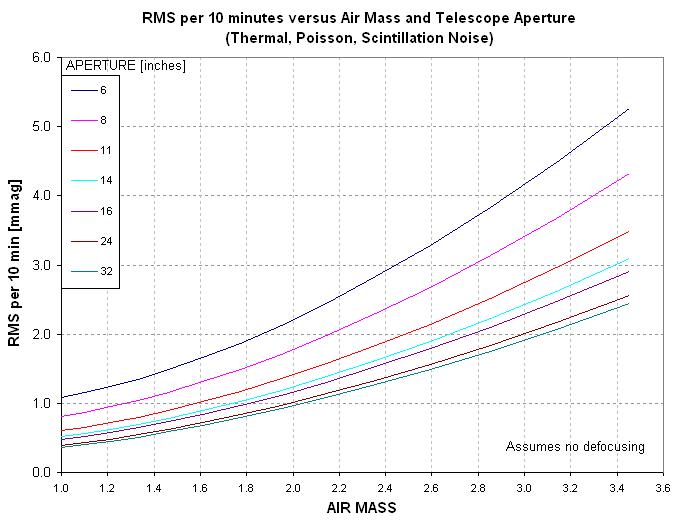
Figure 3. "10-minute RMS" (total of thermal, Poisson and scintillation) versus air mass for a selection of telescope apertures, with duty cycle taken into account.

This last plot is misleading because large apertures will likely defocus and thereby improve their duty cycle, thus recovering some of the lost performance caused by short exposure times that are otherwise required to prevent saturation.

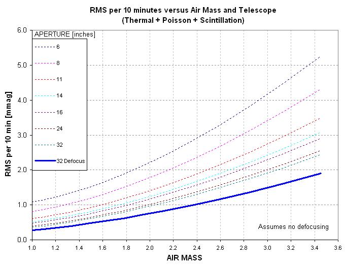
Figure 4. By defooocusing just a little, so that Cmax decreases to ~ 1/3 of the sharp focus value, the total "10-min RMS" for a 32-inch telescope observing HAT-P-13 improves by ~ 30%.

How does this come about, because by defocusing thermal noise should increase since the photometry aperture needs to increase in size?

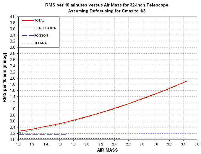
Figure 5. SA 32-inch telescope's noise partitioning shows that scintillation dominates for all air masses but Poisson and thermal noise decrease due to the improved duty cycle.

For apertures greater than ~ 20 inches defocusing will have benefits. They will be modest because the principal component of noise is scintillation, and it only decreases due to defocusing because duty cycle improves somewhat.

This completes the derivation of "10-minute RMS" for a variety of telescope apertures and air mass values.

Return to HAT-P-13 web page

WebMaster: B. Gary.  Nothing on this web page is copyrighted. This site opened:  2010.03.23.  Last Update:  2010.03.23.