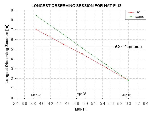
Longest observing session for the rest of the 2010 observing season, defined as the interval for which sun elevation < -11 degrees and HAT-P-13 elevation > 25 degrees.
Links internal to
this web page:
Basic
data
Comments
Table & plots of of AXA transit measurements
Amateur Transit LC's
Professional Transit LC's
OOT LCs
Finder images and all-sky photometry
Two-Planet Perturbations for 2010
Q-Scoring
References
Basic data
RA = 08:39:31.8, DE = +47:21:07
Season = January 28
B = 11.35, V = 10.62, J = 9.328, K = 8.975, B-V = 0.73
+- 0.03; All-sky: B = 11.32 ± 0.10, V
= 10.62 ± 0.08, Rc = 10.22 ± 0.06
HJDo = 4779.92979
(38) & P = 2.916260 (10), (e.g., Schneider listing
in Extrasolar Planets
Encyclopaedia)
HJDo = 4779.92973
(52) & P = 2.9162588 (25) based on AXA data & analysis.
Depth =
9.6 ± 1.0 (CBB-band), 8.0 ± 1.0 (i-band)
Length =
3.23 ± 0.04 hr (i-band & CBB-band)
Fp = 0.30
± 0.15, F2 = 0.78 ±
0.10
b = 0.67
± 0.04
HAT-P-13 is a solar system with at least 3 exoplanets, and the inner-most of these (planet "b") is known to transit with a 2.9-day period. Planet "c" is massive and is in a large and very eccentric orbit. Planet "d" is hypothesized to exist by Winn et al (2010, preprint), and is in an even larger orbit. In late April, 2010 "c" will pass through periastron (closest approach to the star) and if its orbit inclination is approximately the same as for "b" it could also transit. In addition, "c" could distort the gravitational field for "b" in a way that produces transit time variations (TTV) for "b". Both of these effects have been described in recent preprints by Payne and Ford (2010 preprint) and Winn et al (2010 preprint). The possibilities for amateur contributions are described at the bottom of this web page: "Two-Planet Perturbations for 2010" where I show that amateur observers are more likely to contribute to the task of searching for a "c" transit than trying to characterize the "b" TTV anomaly. The AXA will be open for data submissions of two types:
1) OOT: out-of-transit light curves meant for
a search of a possible HAT-P-13c transit, Apr 19 to May 5,
minimum requirement of 4-hours, "10-minute model-referenced
RMS" < 2.0 mmag, and
2) TTV: HAT-P-13b transit light
curves, now to May 10, minimum requirements: 4-hours that include
an ingress and/or egress (preferably both), "10-minute model-referenced
RMS" < 1.5 mmag. (These criteria have been discontinued.)
The first type of data submission will be presented in the "OOT LCs" section of this web page. A table of
submissions will be maintained at the top of that section.
The second type will be processed with the same AXA model-fitting
code used in the past, and the LCs will be displayed in their usual
place on this web page (Amateur Transit LCs).
The section following that one will be maintained in the usual AXA
manner, showing a table of observer submissions, and plots of depth,
length, Fp and F2. In order to keep this database attractive to professionals
(one of the AXA goals), I will only accept data into this archive
that meets the minimum requirements, briefly stated above, and
described in more detail below, at Q-Scoring.
HAT-P-13 is approaching the end of its observing season, which is centered
on January 30. This means that the longest possible observing
session is shrinking by ~ 5 minutes each day. The most likely periastron
passage for "c" is now thought to be April 28 (Apr 26 to Apr 30).
As the following plot shows by Apr 28 the longest possible observation
is already too short for including a complete transit (with an hour
of OOT before ingress and after egress). The implications of this are
discussed in the "Two-Planet Perturbations for
2010" section of this web page.
Longest observing session for the rest of the
2010 observing season, defined as the interval for which sun elevation
< -11 degrees and HAT-P-13 elevation > 25 degrees.
As I have during the 2.5 years that I maintained the AXA, I will be available for a reasonable amount of tutoring via e-mail exchanges on questions from observers who think there's something about their observing procedure, or image processing procedure, that isn't optimum. In the past the most common problem was saturation of either the target star or reference stars (at high elevations, when FWHM is smallest and the risk of saturation is greatest). Also, as I've done in the past, if time permits I will accept sample images for review, by prior agreement, to look for problems and give advice.
All observations of HAT-P-13 submitted to the AXA for HAT-P-13 will be
forwarded to University of Florida (UF) in a standard format
that we have negotiated. One role of the AXA in this project is
to serve as an interface between the UF professional astronomers
and anyone in the community of amateur observers who want to be sure
that their data files are considered for inclusion in the UF analysis.
The UF team has a policy of offering
co-authorship to anyone whose data has sufficient value to be included
in their final analysis and publication. More information about
this special 2.5-month project can be found at the "Two-Planet Perturbations for 2010" section
of this web page.
Also, I will continue the AXA policy of the past
2.5 years by including data files for download by anyone (including
ETD, who have in the past automatically downloaded AXA data files
for inclusion in their database). These files will be in a simple format
close to what is submitted by the observer, whereas the data files
forwarded to the University of Florida astronomers will be rigidly
controlled to a standard format.
Normally, professional astronomers keep their data secret until published
(for funding related reasons), but any professionals wishing for
a more open data sharing relationship are invited to make use of the
AXA for this purpose. All data submitted to the AXA become "public
domain," which means that any professional astronomers wanting to
investigate the presence of a "c" transit, or wanting to constrain
orbit solutions, are free to do so using data files downloaded from
the AXA.
The "season" for OOT observations of HAT-P-13 is April 19 to May 5. This
is the most likely time for a "c" planet transit, if such transits
occur.
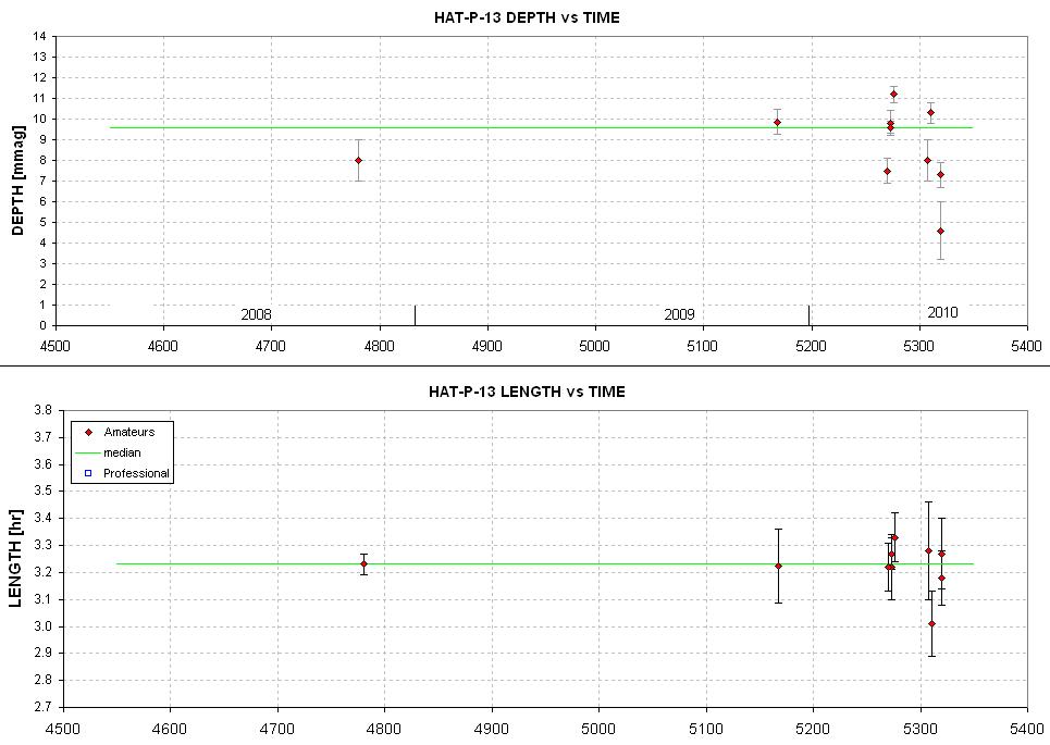
Table & Plots of Amateur Observations ("b transit LCs")
Note the perturbation
that could be produced by HAT-P-13c as it passes by "b".
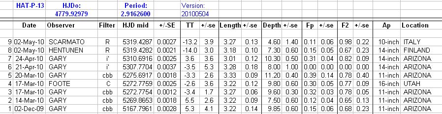
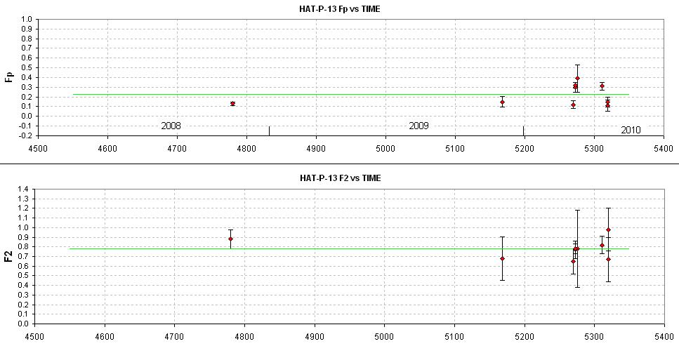
Amateur Light Curves("b transit LCs")
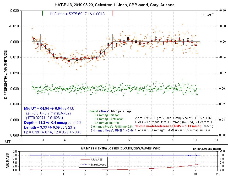
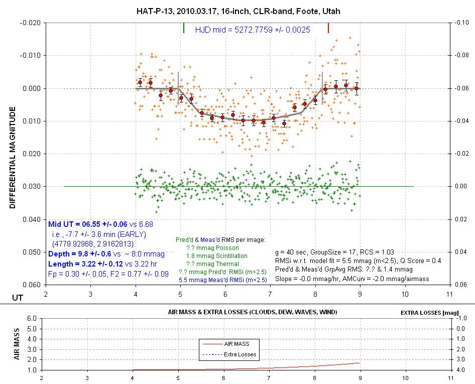
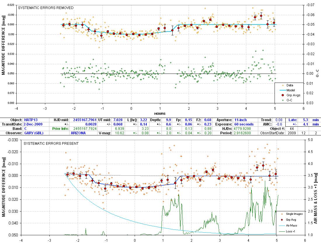
100317-HATP13-Foote-16inch-clr-pro
Note: The CCD cooler (TEC) didn't work during this observing
session, so noise is higher than usual.
9C02GBL Lots of cirrus
clouds.
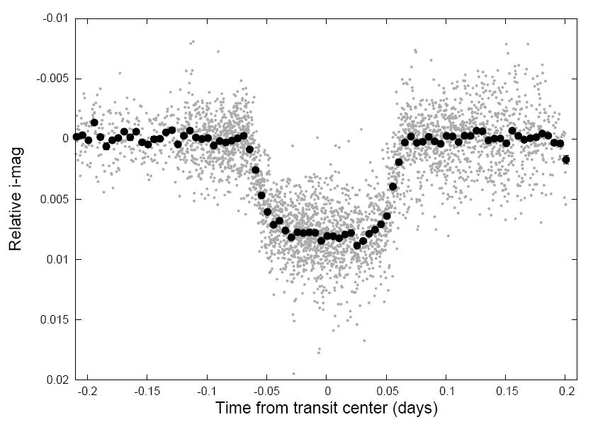
Copied from discovery paper (Bakos et
al, 2009, reference below).
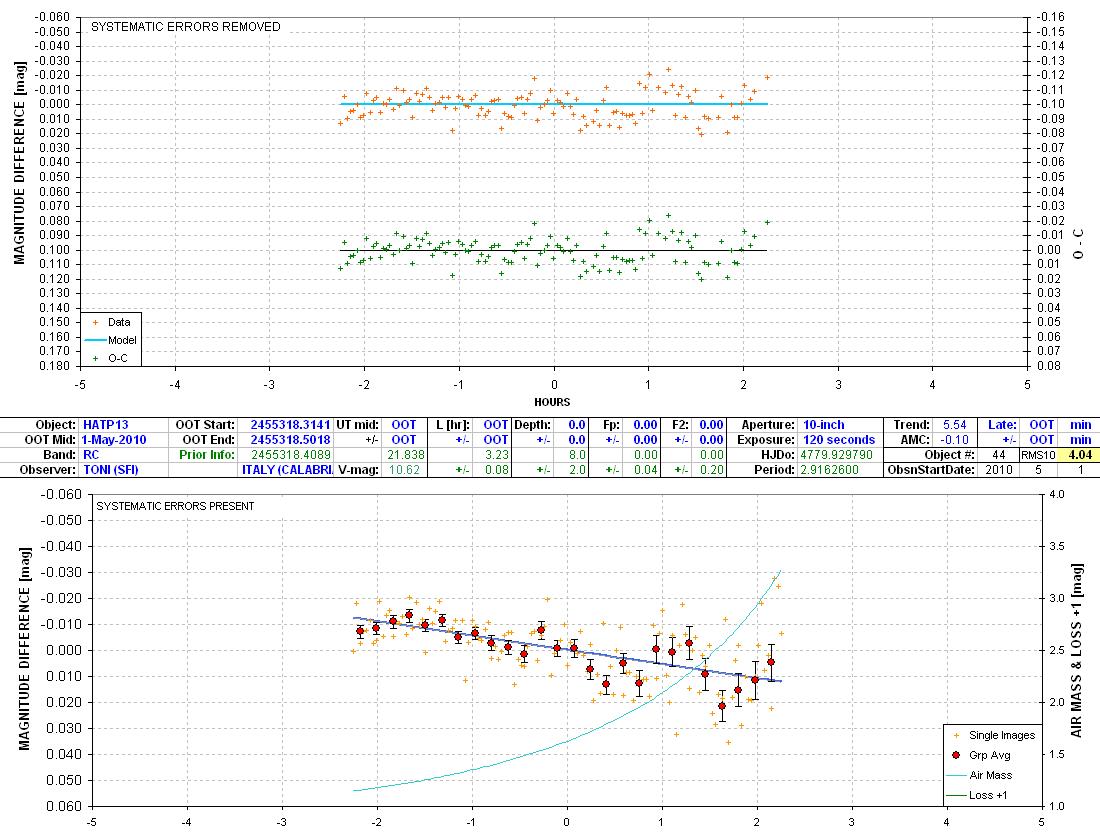
Out-of-Transit (OOT) Light
Curves("c OOT LCs")
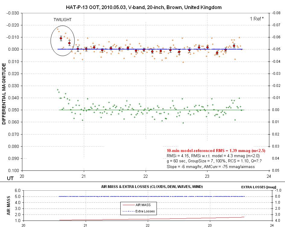
21 2010.05.03 3.0 hr V-band 20-inch
Brown
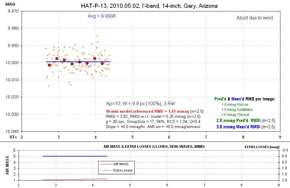
20 2010.05.02 2.0 hr i'-band
14-inch Gary (-0.2 ± 0.7 mmag)
19 2010.05.01 3.6 hr R-band
12-inch Scarmato
18 2010.04.29 4.5 hr R-band
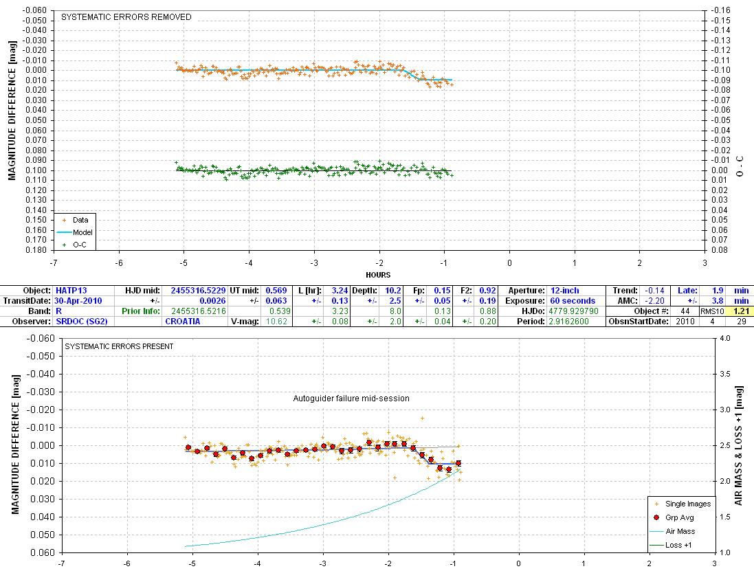
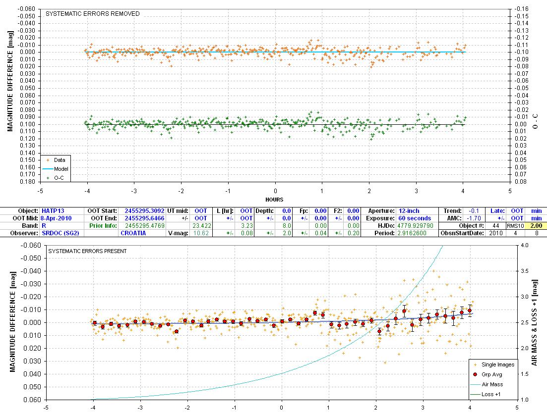
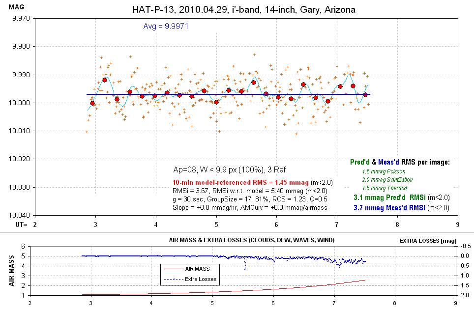
12-inch Srdoc
17 2010.04.29 4.5 hr i'-band
14-inch Gary (-2.5 ± 0.5 mmag)
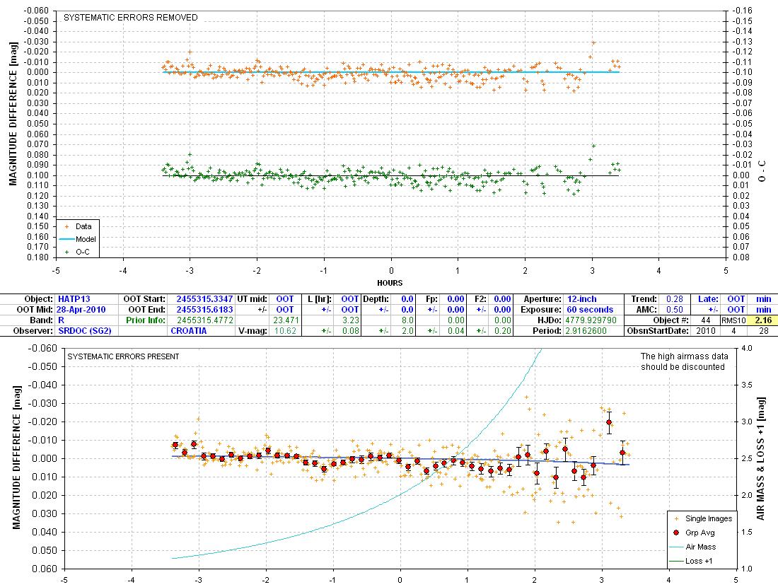
16 2010.04.28 6.5 hr R-band
12-inch Srdoc
15 2010.04.28 5.0 hr i'-band
14-inch Gary (-1.5 ± 0.7 mmag)
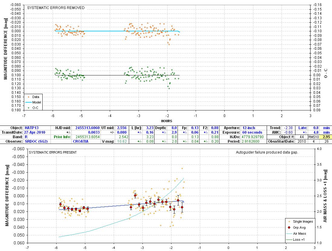
14 2010.04.26 3.0 hr R-band
12-inch Srdoc
13 2010.04.26 5.4 hr i'-band
14-inch Gary (-3.0 ± 0.7 mmag)
12 2010.04.25 6.0 hr i'-band
14-inch Gary (+0.5 ± 0.7 mmag)
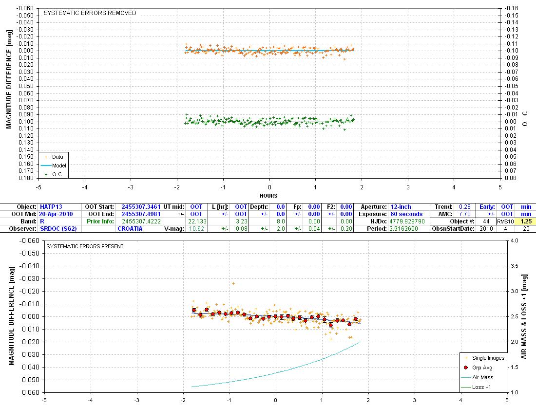
11 2010.04.20 3.6 hr R-band
12-inch Srdoc
10 2010.04.19 3.5 hr R-band
14-inch Hentunen
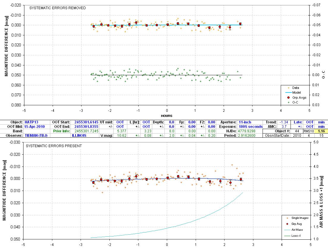
09 2010.04.18 6.0 hr R-band
11-inch Tieman
08 2010.04.17 5.5 hr R-band
11-inch Tieman
07 2010.04.15 5.5 hr R-band
11-inch Tieman
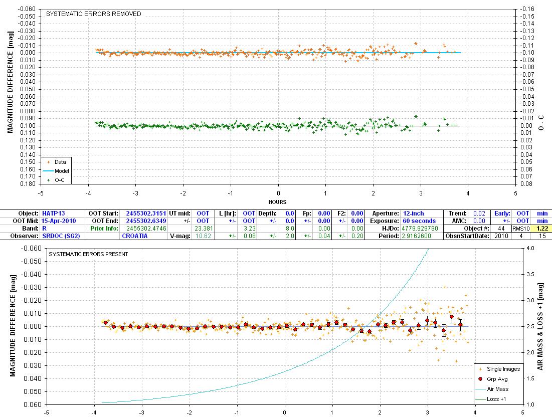
06 2010.04.15 8.0 hr R-band
12-inch Srdoc
05 2010.04.08 8.0 hr R-band
12-inch Srdoc
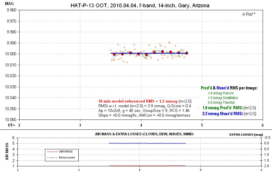
04 2010.04.05 7.5 hr i'-band
14-inch Gary (+0.2 ± 0.6 mmag)
03 2010.04.04 1.1 hr
i'-band 14-inch Gary
(+0.1 ± 1.0 mmag)
02 2010.03.28 3.5 hr R-band
??-inch Ayiomamitis
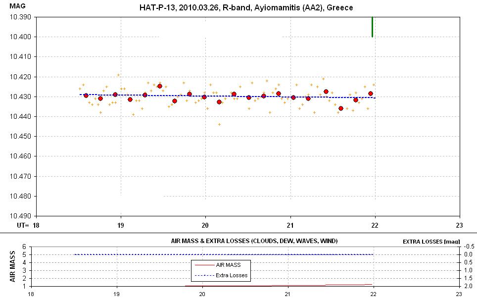
01 2010.03.26 3.5 hr R-band
??-inch Ayiomamitis
Observer: Anthony Ayiomamitis (Greece)
Observer: Daniel Brown (UK)
Observer: Toni Scarmato (Italy)
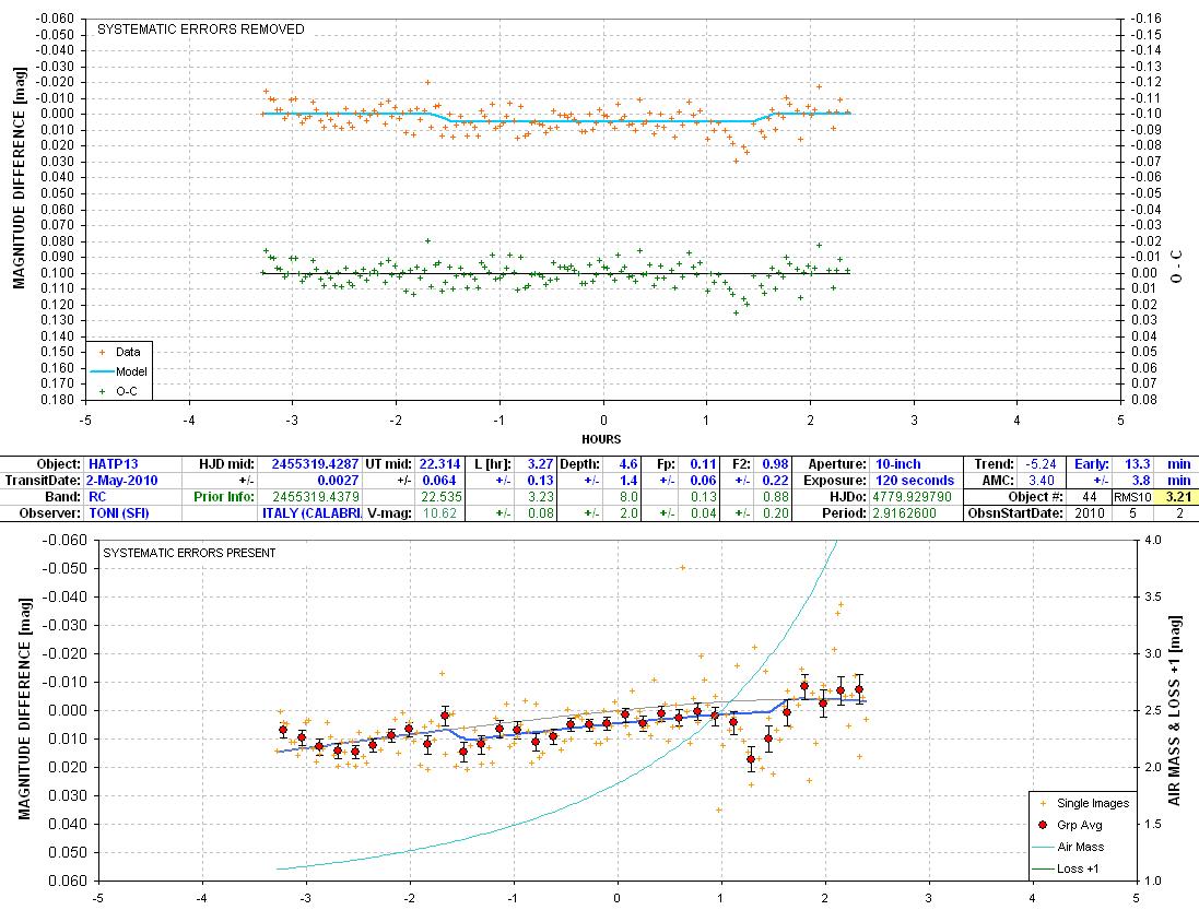
100501-44-SFI Could this be an ingress
feature?
Observer: Gregor Srdoc (Croatia)
Observer: Brian Tieman (Illinois, USA)
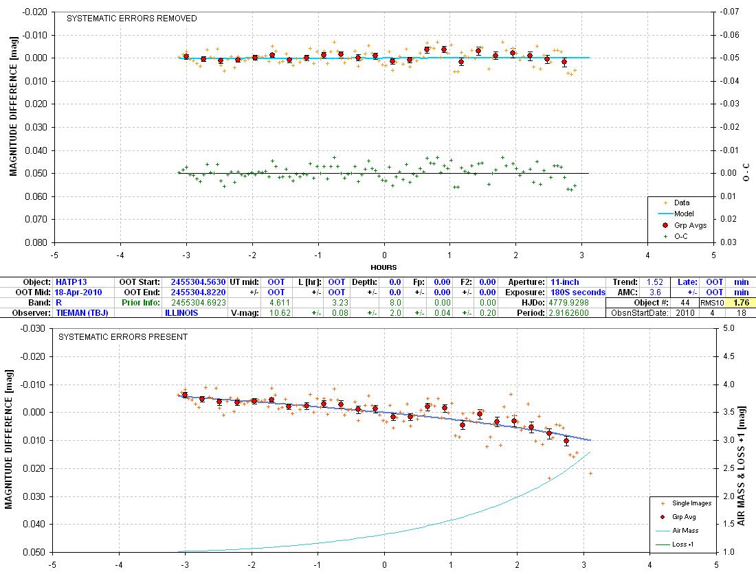
100418-44-TBJ Note:
An ingress begins at 06.94 UT (or 02.3 using the time scale in above
plot).
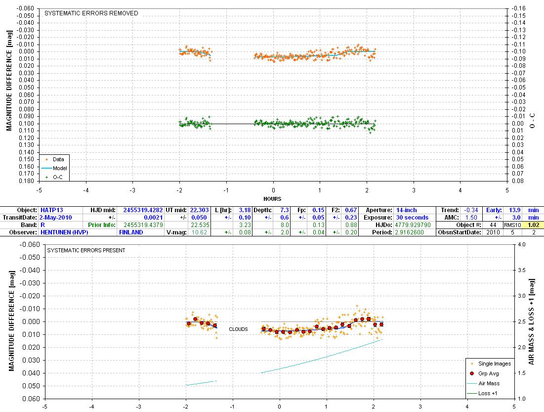
Observer: Veli-Pekka Hentunen (Finland)
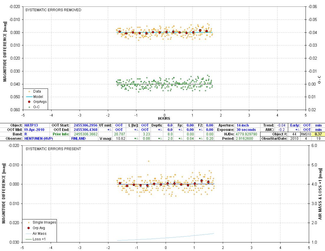
100419-h13-HVP Note
the amazing "10-minute model-referenced RMS" = 0.37 mmag!
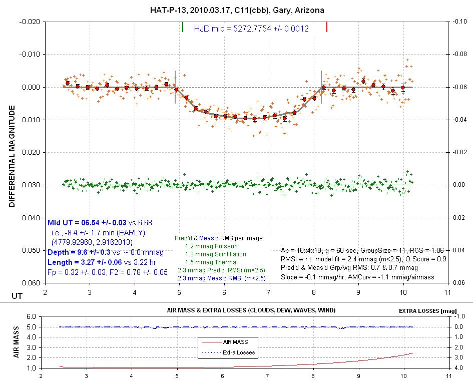
Observer: Bruce Gary (Arizona)
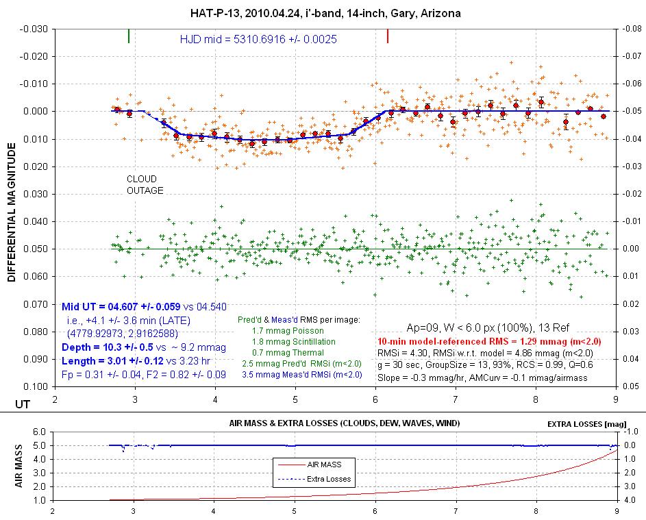
100429-h13-GBL-M14(i')-a08w99-sys
Very windy last half.
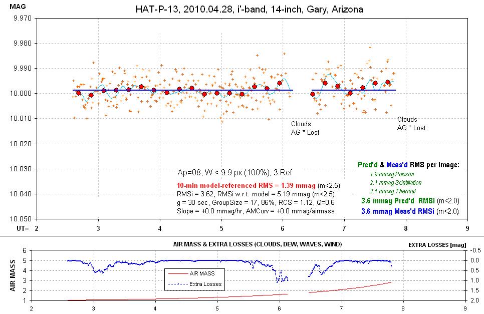
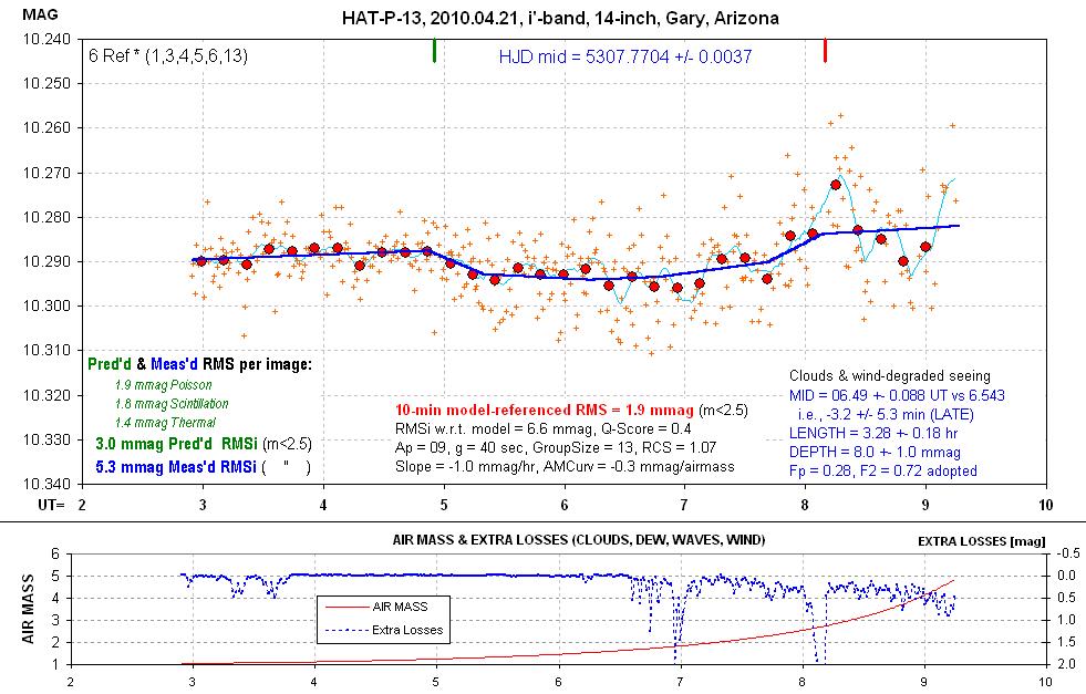
100428-h13-M14(i')-a8w99-sys
Average brightness is till high, by ~ 1.5 mmag.
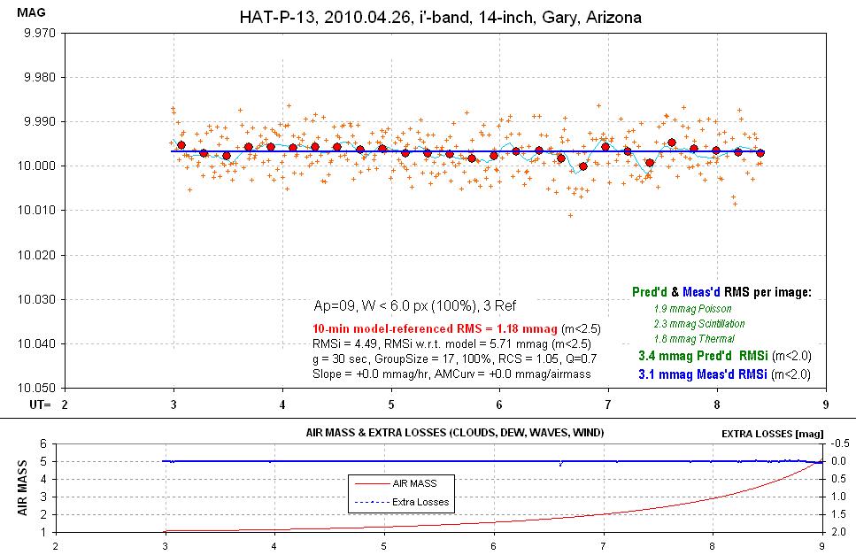
100426-h13-GBL-M14(i')-a09w99-sys
I don't know why the average brightness is 3 mmag higher
than on the other dates. I used the same 3 ref stars to set calibration.
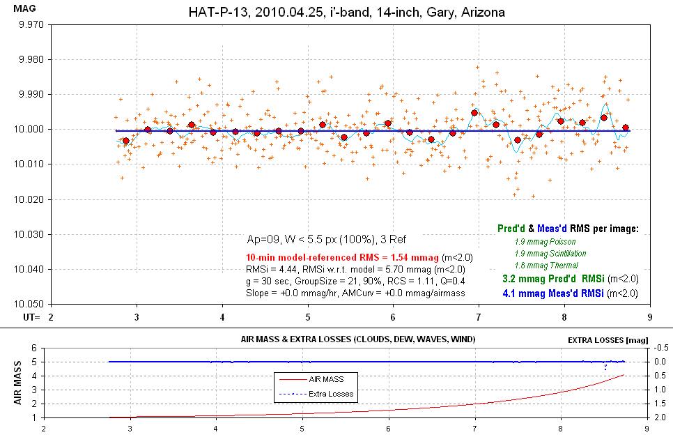
100425-h13-GBL-M14(i')-a09w99-sys
Finder Images and All-sky Photometry
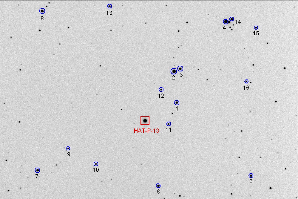
Star numbers for all-sky photometry table,
below. FOV = 22 x 15 'arc, north up, east left.
Preliminary all-sky photometry magnitude results (based on 2010.03.12):
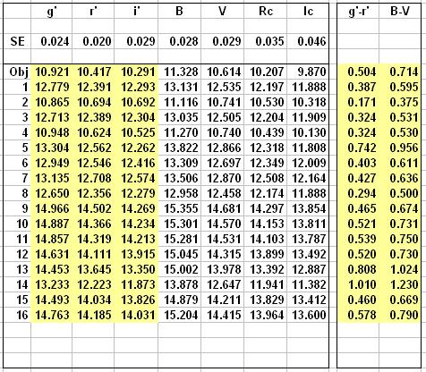
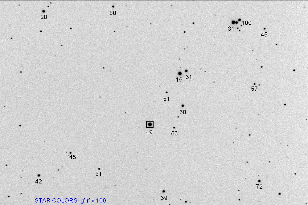
Preliminary all-sky star colors, 100 x (g'-r'),
for use in selecting "same color" reference stars.
Summary of HAT-P-13 all-sky photometry magnitudes.
Normally I do two all-sky observing sessions before declaring
a "final" result so that will also happen in due time.
| Source | B | V | Rc | Ic | g' | r' | i' | B-V | g'-r' | version |
| J=9.328, K=8.975 | 11.10 ± 0.08 | 10.49± 0.05 | 10.15 ± 0.04 | 9.81 ± 0.04 | +0.62 ± 0.10 | |||||
| HAO all-sky (provisional) | 11.328 ± 0.028 | 10.614 ± 0.029 | 10.207 ± 0.035 | 9.870
± 0.146 |
10.921 ± 0.024 | 10.417 ± 0.020 | 10.291 ±
0.029 |
+0.714 ± 0.040 | +0.504 ± 0.031 | 2010.03.12 data |
| HAO all-sky (final) |
Joao Gregorio includes an image annotated with B-V star colors (derived from 2MASS J and K) at this web site: http://atalaia.org/gregorio/hatp13data.php
Two-Planet Perturbations for 2010
This AXA web page has been reactivated in response to a rare observing opportunity during April and May. HAT-P-13 is a 2-planet system (3 planets, according to Winn et al, 2010 preprint), with "b" transiting every 2.9 days and a massive "c" in a highly eccentric orbit having a period ~ 430 days (Payne and Ford, 2010 preprint) or ~ 448 days (Winn et al, 2010 preprint). The Winn et al period is based on more radial velocity data, so their soluton should be more accurate. The inclination of the outer planet could either be approximately coplanar with the inner planet or tilted ~ 45 degrees, according to current observational constraints and theoretical considerations. The Winn et al paper suggests that the "c" (outer) planet orbit is close to being coplanar (i.e., inclination close to 90 degrees), based on their measurements of the Rossiter-McLaughlin effect of "b" transits (calling for the star's spin axis orientation being close to perpendicular to the "b" orbital plane). If indeed the "c" orbit is coplanar with "b" then two interesting scientific goals are feasible: 1) the outer planet might transit (maybe 8% probability), and 2) the inner planet's orbital eccentricity can be measured and used to infer the planet's mass distribution. Both goals might be within reach of advanced amateur exoplanet observers to make useful contributions. This year the "c" periastron date have been estimated to be Apr 16 ± 8.5,6.5 (Payne and Ford, 2010) and Apr 28.7 ± 1.9 based on more radial velocity observations (Winn et al, 2010, though "jitter" assumptions might make this solution optimistic). Greg Laughlin has a good description of this upcoming event posted at his oklo web site: http://oklo.org/ (March 17), and also http://oklo.org/2010/03/25/this-just-in/ and most recently http://oklo.org/2010/03/31/hat-p-13-good-news-and-bad-news/. Here's a depiction of the "b" and "c" orbits that appears at the oklo web site:
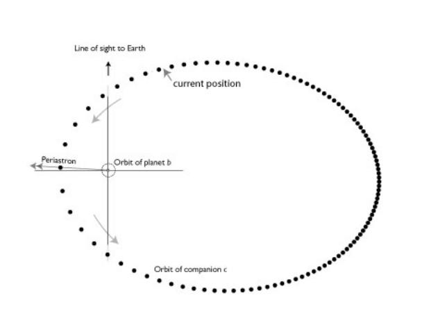
Figure 1. Orbits of HAT-P-13 "b" and "c" showing Earth's line-of-sight
in relation to the "c" periastron (Laughlin, oklo post of March
17).
This observing opportunity repeats every 14.7 months, and next year's
periastron passage (late July) occurs when HAT-P-13 is close to the sun and
can't be observed. Observations are possible in 2012 (mid-October) but are
less favorable than this year's. A good opportunity will occur in January,
2014. The HAT-P-13 "observing season" is centered on January
30. After this date observing sessions become shorter and are now
only 7.0 hours long and shortening by ~ 5 minutes per day. By April
20 they will become shorter than the 5.2 hours needed to obtain a complete
transit (with an hour of OOT before ingress and after egress).
Figure 2. Longest observing session
for the rest of the 2010 observing season, defined as the interval
for which sun elevation < -11 degrees and HAT-P-13 elevation
> 25 degrees.
As described below the challenge of short observing sessions greatly affects
the ability to obtain light curves that can be used to study
the HAT-P-b TTV anomaly. The OOT goal is less affected, and for
this reason I suggest that it become the principal goal for amateurs.
There are two observing goals, corresponding to the two scientific opportunities
mentioned above (accomodating both preprint periods for "c"):
1) out-of-transit (OOT) measurements, from April
9 to May 2, when a "c" transit might occur, and
2) transit timing variations
(TTV) for "b" transits, from now to mid-May.
Both amateur and professional observatories are being requested to participate
in a project being coordinated by astronomers at the University
of Florida (UF). The UF astronomers most involved in this project
are Mathew Payne, Eric Ford and Benjamin Nelson, with Ben Nelson
being the principal coordinator of the observational phase of
the project. I have volunteered to help in coordinating amateur observers
and will reactivate the Amateur Exoplanet Archive (AXA) for amateur
data file submissions of HAT-P-13 observations from now until mid-May.
Other professional astronomers will surely be conducting and coordinating
similar observing programs of HAT-P-13 this year. Data files submitted
to AXA will become "public domain" and will be available for download
and use by anyone.
A. Search for Transit of HAT-P-13c: Apr 9 to May 2, 2010
The other goal for this collaboratiion is to search for a transit of HAT-P-13c by observing during the 15-day interval Apr 9 to May 2 (which is compatible with both the Payne and Ford orbit solution and the Winn et al orbit solution for "c" periastron passage). The observing strategy for this task is simple: observe the same HAT-P-13 star field every clear night, with the same filter (CBB or clear), and process the imags in exactly the same way for every observing session. Image processing should also be stratightforward: decide on a set of reference stars and use them for processing EVERY observing session.
The probability for a transit of "c" is small (somewhere between 1 and 8%). If it occurs it will could have a "length" less than ~ 15 hours. No single observer is likley to notice an ingress or egress feature so any search for the "c" transit will require blending LC segments from many observers. Since the depth for a "c" transit is likely to be ~ 8 to 10 mmag, and since nobody can calibrate their LCs to this accuracy, it will not be necessary to attempt CCD transformation of instrumental magnitudes to standard magnitudes; rather, each observer should use the same set of reference stars (carefully selected, see "Finder..." section on this web page for star colors of nearby stars) and the UF team will determine an OOT offset adjustment for each observer.B. Search for HAT-P-13b TTV: Now to mid-May, 2010
As "c" approaches periastron it will create a slight distortion to the gravitational field expierenced by "b", causing "b" transits to first occur "early" and later to occur "late." This TTV is illustrated by the calculations by Payne and Ford (2010, preprint):
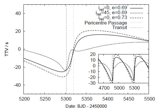
Figure 3. TTV calculations by Payne and Ford (2010 preprint) for
an interval 2010.01.04 to 2010.10.31, showing a TTV variation
of as much as 50 seconds between Apr 4 and Jun 3. Peak-to-peak
TTV anomalies of between 10 and 100 seconds are possible. This
figure is based on the Payne and Ford orbit solution; the Winn et al orbit solution would shift these
plots 12 days to the right.
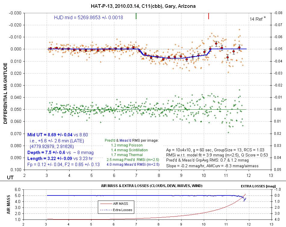
If the peak-to-peak anomaly is ~ 50 seconds (it could range from ~10 to 100 seconds) the TTV for "b" will be difficult for amateurs because of the shallow depth (9 mmag). With my 11-inch Celestron I have been able to achieve a mid-transit accuracy ~ 100 second for a complete transit occuring at high elevations (2010.03.17), which illustrates the challenge for amateurs to detect the expected TTV anomaly. If many amateurs produce LCs of comparable accuracy, however, it might be possible for their average to be useful in detecting this level of TTV. Here's a TTV plot showing the anomaly in relation to both professional and amateur observations.
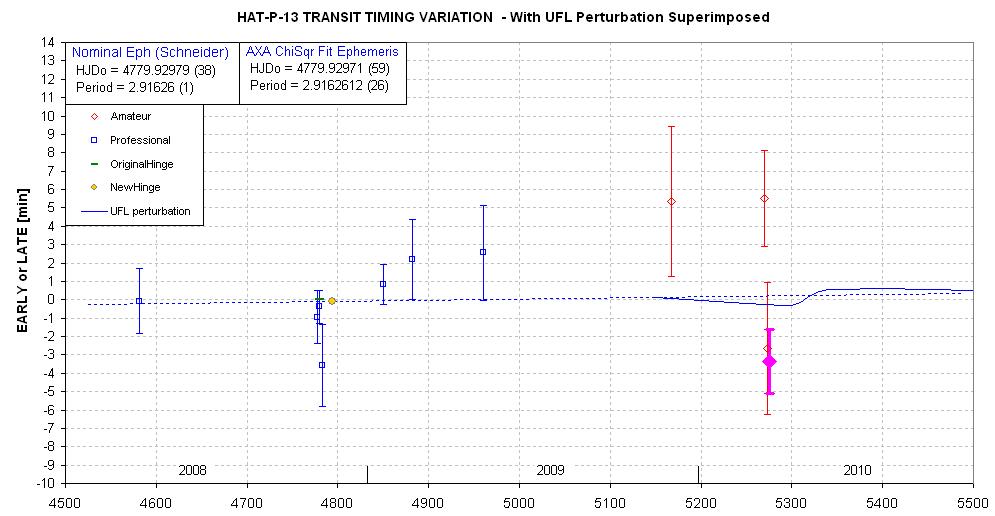
Figure 2. TTV plot as of 2010.03.17,
showing both professional and amateur observations. The
thick purple datum was made with a 11-inch telescope and exhibits
a mid-transit time SE of 100 sec, which represents a goal for
future observations. This figure is based
on the Payne and Ford orbit solution; the Winn et al orbit solution would shift
these plots 12 days to the right.
It is clear that only good quality LCs are going to be useful for this ambitious task. To estimate feasibility of detecting the above 50 second peak-to-peak TTV feature I used the 18 transit observations that I've conducted during the past 2.5 months using my Celestron 11-inch and Meade 14-inch telescopes to investigate the relationship between mid-transit time accuracy versus two independent variables: transit depth and star flux (taking the filter and telescope aperture into account). The result of this study is shown in the next plot.
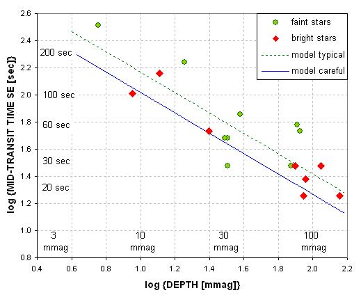
Figure 3. Relationship between
TTV accuracy and transit depth when using 11-inch and 14-inch
telescopes. The blue model line corresponds to "carefully" processed
measurements under good observing conditions (high elevation during
entire transit). My HAT-P-3 measurement on 2010.03.17
is the "bright star" symbol just below the "model careful"
line, on the left. The transition from "faint" to "bright" corresponds
to a star having R-mag = 10.5 while using a CBB filter with a 11-inch
telescope.
Surprisingly, the strongest correlation of TTV SE is with transit depth, not star brightness. This would suggest that seeking improved TTV SE by using larger telescope apertures has slow payoffs. Additional theoretical analysis indicates that much of the scatter in the above plot is due to the importance of scintillation that renders high air mass ingress and egress observations much noiser than near-zenith observations (see below). When HAT-P-13 at high elevations carefully processed images should produce the following mid-transit SEs:
11-inch 100 sec
16-inch
80 sec
24-inch
60 sec
32-inch
50 sec
For apertures larger than ~ 20 inches I recommend using a CBB-filter and defocusing in order to maintain a reasonable duty cycle ( > 80% of telescope time spent exposing).
If four such observations are made for one event, then divide the mid-transit SE numbers in the above table by 2. It might be possible to obtain four quality measurements for events visible in Europe because of the many good amateur exoplanet observers at those longitudes. Thus, averaging a dozen good mid-transit time measurements for events visible in Europe might be possible, and they could lead to an SE of ~ 20 or 30 seconds per transit event. At any one longitude complete transits are visible 3 days apart at intervals of ~ 36 days during the HAT-P-13's observing season (see next table). Thus, European observers may be able to characterize a TTV value for a 3-day interval with an accuracy of ~ 20 sec. Fewer experienced amateur exoplanet observers are located at American longitudes so professionals will have a greater responsilibity for dates corresponding to these longitudes.
The following three tables are my calculations for transit visibility for Greece, Portugal, Florida and Arizona.
![]()
Figure 4. HAT-P-13 observing opportunities
for observers in Greece.
![]()
Figure 5. HAT-P-13 observing opportunities
for observers in Portugal.
![]()
Figure 6. HAT-P-13 observing opportunities
for observers in Florida and Pennsylvania (East Coast of USA).
![]()
Figure 7. HAT-P-13 observing opportunities
for observers in Arizona.
Based on the above tables it is possible to specify on a TTV plot when complete transits are visible for observers at the four longitudes represented by the tables.
Figure 8a. Illustration
of when observers at different longitudes can observe a complete
transit of HAT-P-13 using the Payyne and Ford (2010 preprint) orbit
solution. After mid-May observing sessions will
be too short to capture both ingress and egress (for all observing sites).
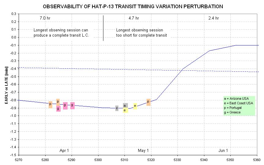
Figure 8b. Illustration
of when observers at different longitudes can observe a complete
transit of HAT-P-13 using the Winn et al,
2010 orbit solution. Numbers at the top show the longest possible
observing session, and for JD4 > 5202 no observers on Earth surface
will be able to observe a complete transit, requiring ~ 5.2 hours
(3.23 hour from ingress to egress, plus an hour of OOT on each side).
The two figures, above, show that there are a few opportunities for groups in Europe and America to establish a "pre-upswing" timing level but there are no opportunities to observe the highest part of the anomaly. If the Payne and Ford orbit is correct (cf, Fig. 8a), then some of the "upswing" part of the anomaly can be observed by partial transit observing sessions (i.e., including either ingress or egress, but not both) because the upswing begins after longest possible observing sessions are too short for including a complete transit (cf, Fig. 8b). If the Winn et al orbit is correct then there will be no opportunities for observing any of the upswing or following part of the anomaly. Transit length is 3.23 hours, and if an hour of OOT is needed before ingress, and after egress, then an observing session of 5.2 hours (at high elevations) is needed to obtain a high quality LC. As described in the "Observing Situation Considerations" section, below, this will not be possible after ~ April 20 (JD4 = 5306). Accordingly, none of the TTV anomaly can be observed under conditions good enough to evaluate the amplitude or shape of the TTV anomaly in 2010. This task will have to wait until the 2014 January periastron passage of HAT-P-13c.
It has been suggested to
me that LCs that include only an ingress, or egress, can be used
to establish a mid-transit time provided transit length (and shape)
are well established. I've done this for a XO-1 TTV study, and
I have serious reservations about the approach. In my experience
systematic effects are are almost always present in amateur LCs (due
to the high extinction at amateur observing sites, which are compounded
by the use of high throughput filters, such as CLR or CBB, that are
required when using small telescope apertures). Without an hour of OOT
before ingress and after egress the air mass curvature effect is difficult
to establish, and correct for. Professional telescopes have sufficient
aperture for using such filters as z', Ic, NIR, Rc and V, all of which
are narrow enough to greatly reduce air mass curvature effects. Therefore,
I think the professional observers using professional observatories are
in a much better position to characterize the TTV anomaly than amateurs.
Longest
Observing Session Limitations
HAT-P-13b transit length is 3.23 hours, and since it is
important to obtain at least an hour of OOT observations before
ingress and after egress, the minimum observing session length
for a complete transit is ~ 5.2 hours.
The HAT-P-13 "observing season" is centered on January
30. That's when HAT-P-13 passes through the meridian (is highest
in the sky) at local midnight, when an observing session can be longer than at any other
date. On that date HAT-P-13 can be observed for 10.4 hours
from most latitudes. At the present time (March
26), HAT-P-13 can be observed above 25 degrees elevation for 7.0
hours from my latitude (+31 deg). At a European latitude (51 degrees,
Belgium) the longest observing session could be 8.4 hours. On April
15 the longest observing session from my site will be 5.5 hours. At
a European site it will be 6.5 hours. At the most-likely
"c" periastron passage, April 28, the longest observing sessions
will be 4.5 and 5.0 hours. On May 15 the lengths are 3.1 and 3.5 hours.
On May 31 they are 1.8 and 1.8 hrs. Here's a plot of these numbers.
Figure 9. HAT-P-13 longest possible observing
session versus date for two sites, HAO (Hereford Arizona Observatory,
lat = +31.4 deg) and Belgium (lat = +51 deg). The longest observing
session is determined according to two conditions: 1) sun's elevation
< -11 degrees, and 2) HAT-P-13 elevation > 25 degrees. The 5.2-hour
requirement allows for 1 hour of OOT before ingress and after egress.
Complete transit observations of HAT-P-13b transits will
not be possible after ~ Apr 20, which occurs before the most
likely periastron passage of planet "c". Incidentally, full moon occurs on April 28, when HAT-P-13
will be ~ 97 degrees away from the full moon.
I conclude that the complete TTV anomaly of 2010 will not
be observable from Earth surface-based observatories!
However, there is merit in trying to establish a transit
timing value for the early phase of the TTV anomaly, which is
already in progress. If a good ephemeris can be established for the
pre-periastron passage date it can be compared with an ephemeris
that applies to the late 2010 dates. There should be differences that
are almost as great as the peak-to-peak TTV of the complete 2010 anomaly.
"Q-scoring" refers to the considerations I'll use in determining if a
submitted data file is acceptable for inclusion in the AXA HAT-P-13 archive
for eventual transfer to UF in a standard format. The scoring is slightly
different for the two types of obervations, TTV and OOT.
Data submissions to the AXA will be of two types:
1) TTV, or HAT-P-13b transit
light curves, with the following minimum requirements: observing
session > 4 hours, must include both ingress and egress, "10-minute
model-referenced RMS" < 1.5 mmag. Observing dates between
now and June 12.
2) OOT (out-of-transit)
light curves meant for a search of a possible HAT-P-13c transit,
with the following minimum requirements: observing session >
4-hours, and "10-minute model-referenced RMS" < 2.0 mmag
(model fit will usually be a straight line with solved-for slope).
Observing dates must be between Apr 12 and May 2.
To illustrate what a "b transit LC" looks like that meets the above TTV goal requirement, consider the following 8-hour LC that has a "10-minute model-referenced RMS" = 0.8 mmag:
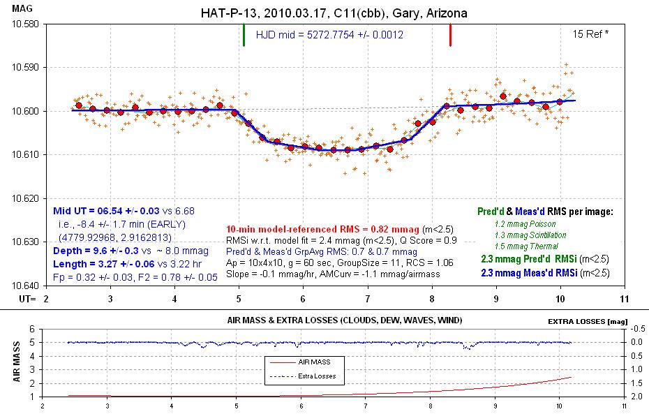
Figure 10. HAT-P-13 LC made with
a 11-inch Celestron and CBB-filter, that meets the requirement
for inclusion in the AXA archive. The RMS for individual 60-second
exposures is 2.4 mmag when measured with respect to a model fit.
Considering that images are 71 seconds apart the "10-minute model-referenced
RMS" is 0.8 mmag. This meets the requirement of 1.5 mmag by a factor
2.
Larger aperture telescopes should be able to provide a better quality than
this one because they afford lower Poisson noise (per unit observing time)
and lower scintillation (per unit observing time). The third component, thermal
noise, isn't directly related to telescope aperture because it is determined
almost entirely by the CCD. In my experience using a 11-inch Celestron Poisson
and scintillation noise levels are comparable near zenith, while scintillation
dominates at high air masses. For laerger apertures all three sources of
noise will be comparable near zenith, but scintillation dominates as soon
as air mass exceeds ~ 1.2 (as derived at this link).
Telescopes larger than ~ 20 inches that are
used with a CBB (or CLR) filter will have to reduce exposure
time from the 60 seconds used in the above example, or defocus,
or use a R- or Ic-band filter. Otherwise, images will be at risk
of saturating HAT-P-13. If the exposure time is very short, duty
cycle suffers, and it is important to keep duty cycle (fraction of
observing time spent exposing) above ~ 75%. It is probably the case that
large aperture telescopes should never employ binning because this just
brings you closer to saturation (time saved with shorter downloads is
not worth the time lost by downloading more frequently).
In Q-scoring the TTV and OOT data files I will process them using an auto-fit
code that I've been using for over a year, and when I notice
that the beginning or end of an observing session can be improved
by deleting data I will try to improve the Q-score by making trial
delections. The LC in Fig. 9 might have benefitted from deleting
data near the end; this "improving by pruning" data will be a subjective
process unless I figure out a way to automate it.
The OOT observations must be made with careful placement of the FOV in
the same star field location on all observing sessions. Autoguiding
is a very important way to reduce the systematic effects related
to imperfect flat fields. In selecting which stars to use for
reference (the same stars must be used for reference for all submisions)
consider the goal of using "same color" stars. For example, if
your FOV is similar to that shown in the "Finder Images..." section
above (internal link) you will note that
HAT-P-13 has a star color of g'-r' = 0.49. Nearby stars that are both
bright and have a similar color could be stars # 1, 6 and 7. Another method
for selecting reference stars is to experiment with various selections.
This is what I do, using a spreadsheet designed for this purpose.
When all OOT data files have been transferred to UF someone there
will determine an offset for each observer that puts the magnitudes
on a standard scale. In searching for a a transit feature it will
be possible to superimpose all such adjusted LC segments, from all
observers.
There's a good reason for using "model-referenced" RMS for evaluating
data quality. Systematic errors will usually produce distortions that acnnot
be fit by a transit model. For example, if you're observing with a German
Equatorial mount you will have to perform a meridian flip during a 5-hour
oberving session, and the star locations on the CCD will change. Any imperfections
in the flat field (and no flat field can be perfect, unless the filter is
very narrow) will produce an offset at flip time. No transit model can match
such a feature, and if this offset isn't corrected before model-fitting the
"model-referenced RMS" will suffer. I am able to solve for this if you tell
me the time of the flip, so if your aa GEM observer, add this in a comment
line of the data file header.
Data format requirements for submitting to
the AXA are explained at http://brucegary.net/AXA/x.htm#Observation_Submission_Format
Many other tips can be found at the AXA home page: http://brucegary.net/AXA/x.htm
I encourage practice observing sessions with HAT-P-13 before the dates
of interest. OOT observing can be the most useful since they
will show the presence of any systematic errors much more clearly
than transit observations.
[more for this section coming]
My recently published book Exoplanet Observing
for Amateurs, Second Edition (sold by Adirondack) has many
suggestions for observing exoplanets for both the TTV and OOT
objectives. It can be purchased at: http://www.astrovid.com/ for $40
(I have no financial stake in book sales).
Noise Source Partitioning
There are three principal sources of noise for target magnitudes derived
from each image. A better way to express this is to calculate
the "10-minute RMS" that would be expected for a specific observing
situation if systematic effects were not present. In the following
plot I've chosen HAT-P-13 for the target and Star #2 (see above finder
image) as the single reference. I've specified exposure times of
60 seconds (or shorter if required to not saturate), and I've assumed
a "download plus settle time" of 10 seconds.
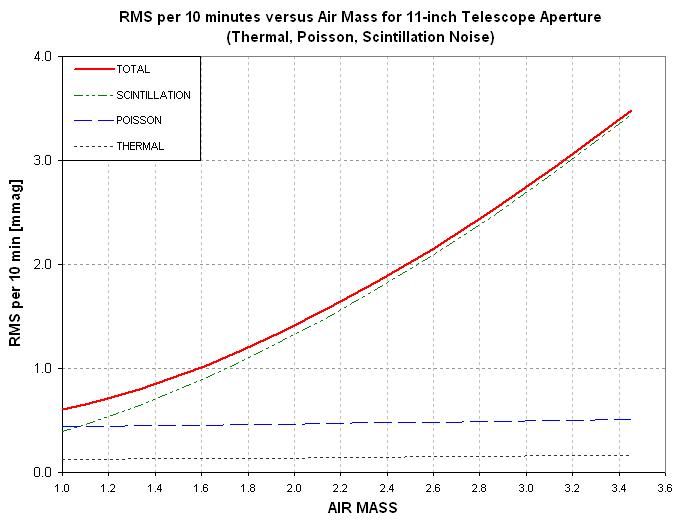
Figure 11. "10-minute RMS" for the three
noise sources versus air mass for a 11-inch telescope, with duty
cycle taken into account.
This plot shows that near zenith Poisson and scintillation noise are comparable
(for an 11-inch telescope). However, beyond air mass ~ 1.5
scintillation dominates. Thermal noise is never dominant.
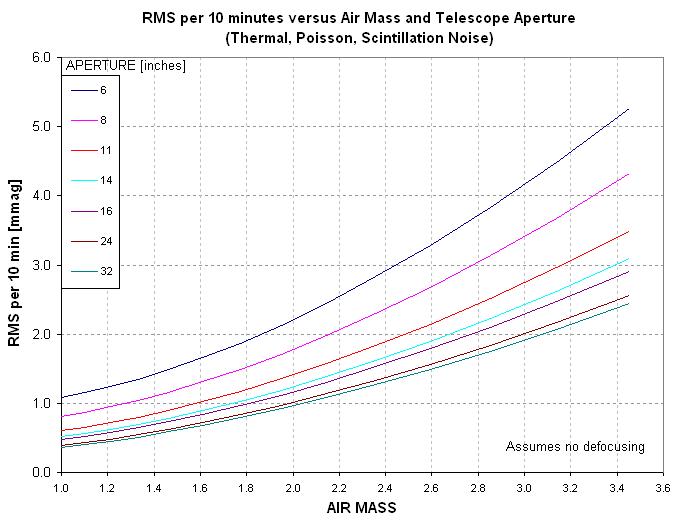
Figure 12. "10-minute RMS" (total of
thermal, Poisson and scintillation) versus air mass for a selection
of telescope apertures, with duty cycle taken into account.
This last plot is misleading because large apertures will likely defocus
and thereby improve their duty cycle, thus recovering some
of the lost performance caused by short exposure times that are
otherwise required to prevent saturation.
For large apertures a modest payoff can be had by defocusing so that duty
cycle can remain high, as the next figure illustrates for a 32-inch
telescope.
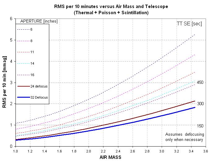
Figure 13. By defocusing so that Cmax
decreases to ~ 1/3 of its sharp focus value for 24-inch, and
1/4 of sharp focus value for 32-inch, longer exposure times are
permitted and duty cycle can remain high. This leads to a ~ 30% improvement
in total "10-min RMS" for a 32-inch telescope. Defocusing isn't required
for apertures < ~ 20 inches (for HAT-P-13, using a CBB filter). On
the right are estimated mid-transit timing SE estimates.
A detailed description of how the last three plots were calculated is given
at this link: 10-minute RMS Noise Levels Derivation
It should be kept in mind that the above plots are close to "most optimistic"
since they don't allow for systematic effects. That's the difference
between "10-minute model-referenced RMS" and "10-minute RMS."
Another thing to keep in mind is that scintillation varies, and one night
might be unusually good and the next night might be quite bad.
It all depends on conditions at the tropopause (11 to 16 km overhead).
Jet streams are "bad" and jigh pressure systems are "good."
What's the effect of "10-minute RMS" on HAT-P-13 mid-transit time SE? Ford
and Gaudi, 2006 showed that mid-transit time SE is proportional to what I'm
calling "10-minute RMS" (provided systematics are small). So let's "scale"
my high quality measurement (small systematics) of 2010.03.17
where "10-min RMS" = 0.82 mmag for an average air mass of 1.33.
My measured mid-transit time SE = 100 sec at a time when transit
was at an air mass ~ 1.15. According to Fig. 10 I should have measured
0.7 mmag at this air mass, and this is compatible with what I measured
for the entire light curve. I therefore suggest the following relationship
for HAT-P-13 observations with a CBB-filter:
Mid-transit timing SE [seconds] = 150 × "10-minute
model-referenced RMS [mmag] at transit"
If this is a valid relationship then we can use the right side of Fig.
12 to estimates mid-transit timing SE. Whether a transit occurs
at air mass ~ 1.00 versus 2.00 makes a big difference, especially
for large apertures (because their error budget is dominated by scintillation).
We are now in a position to answer the question: How small an aperture
can be used to provide useful constraints on the hypothesized
TTV anomaly during April? Let's assume that ~10 measurements are
made at each epoch with a telescope having a given aperture. They
will have a model constraining effect equivalent to a TT timing SE
~ 1/3 of that for a single measurement. For example, a 11-inch telescope
observing at air mass 1.20 on 10 occasions will have an equivalent
TT SE = 30 sec. If orbital constraints now permit a peak-to-peak
change of ~ 100 sec, then two such sets of 10 measurements will have
a difference of ~ half this amount. A 2-sigma constraint is barely
significant. Only in combination with other measurements will this be
useful.
A 6-inch aperture is predicted to produce LCs with TT SE = 180 sec, assuming air mass ~ 1.20. This extra 80% of uncertainty renders the measurement of marginal usefulness.
It is noteworthy that a 6-inch telescope observation of ingress and egress
near zenith is expected to have the same TT timing SE as a 32-inch
telescope observing when ingress and egress occur at an air mass
of ~ 2.6. The "message" here is that it is important to observe
HAT-P-13 when it is "high in the sky."
Concluding Remark
There are two goals for the Apr/May/Jun observing season of HAT-P-13. The
easier one is to make OOT observations on any date between Apr 9 to May 2.
They must be for at least 4 hours, and the same FOV placement is required
for all observing sessions so that the same reference stars can
be used for processing all image sets.
The more difficult task is to observe transits between now and Jun 24.
This will only be worth doing if you have a telescope with an
aperture of at least 11 inches. If you don't use a CBB-filter,
and have to observe CLR, be prepared for high systematics (due to
the fact that HAT-P-13 is redder than all other nearby stars that
are within 2.1 magnitudes as bright). If you use a R-band filter, don't
bother observing transits unless you have 20-inch or larger aperture.
Observations below an elevation of ~ 25 degrees will be severely degraded
by scintillation.
Data files should be attached to an e-mail sent to axa@brucegary.net. My
e-mail is 123@brucegary.net (or "anything"@brucegary.net).
Q1. What's lowest elevation for useful HAT-P-13 data?
A1. Scintillation grows with air mass and with
my 11-inch telescope the scintillation component of noise renders
data below ~ 20 degrees unusable. For larger apertures it should
be possible to work lower because scintillation decreases with
aperture (as 1/D2/3).
Q2. Is it OK to use just one reference star?
A2. It's OK, but it sure isn't optimum! I typically
use 10 to 20 reference stars. Determining the optimum subset
of stars available for reference is difficult, and is one of the
principal tricks to learn for achieving good quality LCs.
Q3. What's the smallest aperture telescope that can be used to provide
useful OOT measurements for searching for the possible transit
of exoplanet "c"?
A3. About 6 inches.
Q4. What's the smallest aperture telescope that can provide useful transit
timing information?
A4. About 11 or 12 inches.
Discovery paper: Bakos et al, 2009: http://arxiv.org/abs/0907.3525
Return to calling web page AXA
____________________________________________________________________
WebMaster: Bruce
L. Gary. Nothing
on this web page is copyrighted.
This site opened: 2009.07.22. Last Update: 2010.06.24