EXOPLANET OBSERVING TUTORIAL
This
web page is meant to help new observers conduct observations of
exoplanet systems. However, it is already superceded by my book Exoplanet Observing for Amateurs,
which should be available for purchase in the Fall, 2007. Since this web page does cover some of the basics it may have value for beginning exoplanet observers and I will leave it up for
now. Until the book is available for purchase you can preview some of the more advanced concepts at my other exoplanet
observing tutorials, listed below:
XO-3 observations (coming as soon as RA/Dec coordinates are in the public domain)
XO-2 observations
XO-1 observations
Artificial Star Photometry
Interpreting Transit Light Curve
Transit Systematics (similar to what's in forthcoming book)
Links internal to this web page:
Introduction
Overview
for Observing Strategy
Reference Stars
Flat Frames
Hardware Considerations
Observing Procedure
Data Reduction
Dealing
With Interfering Stars
Data Analysis
Non-Transit
"Wander" Observations
Example Results:
TrES-1
Miscellaneous Links
Introduction
Exoplanet observing involves "differential photometry" of a star field
for a series of closely-spaced images taken during many hours, and
perhaps repeated for several nights. The objective is to measure the
ratio of the exoplanet star's brightness relative to one or more
"reference stars" (also referred to as "comp stars" by the AAVSO). The
relative brightness of the exoplanet star is plotted as magnitude
versus time (a light curve) with the hope that this plot will show a
slight fade, such as 1.4% (HD209458) or 2.5% (TrES-1), during the
expected time an orbiting planet transits in front of the star.
The transit event may last ~2 hours.
It has been shown that telescopes as small as 4 inches can be used to
detect such transit fades. I had no trouble detecting HD209458 in
August, 2001 using a 10-inch Meade LX200 and SBIG ST-8E CCD camera. I
now use a Celestron CGE-1400 (14-inch Schmidth-Cassegrain) and a
USB-upgraded ST-8XE CCD. With the 10-inch Meade I was able to achieve
20-minute precision of ~3.4 milli-magnitude, whereas with the 14-inch
Celestron I now can achieve 1 or 2 milli-magnitude precision for
5-minute
averages. Since these precision values are much smaller than the
predicted fade of 19 milli-magnitude (HD209458) and 25 milli-magnitude
(TrES-1) it is definitely possible for an amateur with modest hardware
to detect and even characterize the shape of exoplanet transits.
(For a quick peek at my TrES-1 transit light curves go to http://brucegary.net/TrES-1/x.htm
)
Overview of Exoplanet Observing
Stragegy
My philosophy for observing exoplanet transits can be summarized
with the following two rules:
1) have a good flat frame, and
2) keep the star field at the same approximate
location on the imaging chip for the entire observing session.
If Rule 2 could be observed perfectly, Rule 1 would not be
necessary. Since you should assume that there will always be some drift
of the star field, even at the level of a few pixels, it is prudent to
observe Rule 1.
Conversely, if Rule 1 could be observed perfectly, Rule 2 would not
be necessary. But since it is not humanly possible to obtain a perfect
flat frame it is prudent to observe Rule 2.
The over-riding concept for these two rules is to maintain a
constant observed ratio between the target star and all reference stars
for the condition when the target and reference stars do not vary.
I suppose I should add Rule 3, which is to use a filter. This will
minimize any extinction-related effects, due either to air mass changes
or atmosphere changes. If all reference stars and the target star had
the ssame color then this rule would not be necessary. But since all
stars have different colors it is prudent to observe this Rule 3.
Reference
Stars
It's not necessary to strive for good absolute accuracy of an exoplanet
transit if your goal is to detect the light curve using your own
equipment. It's only when your measurements are to be combined with
those by others that an attempt to achieve moderately good photometric
accuracy is helpful. Here's an image showing three reference stars for
exoplanet TrES-1 when an R-band filter is used.
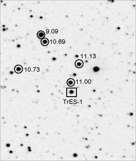
Figure 1. Example of stars suggested for use as
reference stars when using an R-band filter for differential photometry
of TrES-1. FOV = 10.8 x 12.7 'arc, north up, east left.
Notice that for this exoplanet all refernce stars are about as bright
as TrES-1. If only one reference star were used it would add ~40%
additional "stochastic noise" to the brightness measurement of TrES-1
compared with the situation of using a much brighter reference star.
Therefore, for this exoplanet it is important to make use of at least
these three reference stars. This will reduce the stochastic component
of TrES-1 brightness uncertainty to almost that which could be achieved
by having a much brighter reference star.
So far there are only two exoplanets with known transits (that are
observable by amateurs), and for each one there are calibrated
reference stars nearby. If a future exoplanet is discovered that does
not have suitably calibrated reference stars it will surely be
supported by all-sky photometrists quickly, so lacking suitable
reference stars is not likely to be a problem for amateur exoplanet
observers.
Flat Frames
Flat frames is an art that every photometrist should attempt to
master. I don't know if anyone is capable of mastering this art, but
I'll give some tips.
My favorite flat frame trick is to use a "Double T-shirt Cover" that
fits over the aperture and point to zenith at sunset for a series of
flat frame exposures. The T-shirts allow long exposures without the
nuisance of stars showing up. One T-shirt was inadequate, so I use two.
The telescope's f-ratio will determine when exposures can be made. You
want to keep the maximum counts for each flat frame within the linear
region to avoid saturation effects. For my SBIG non-anti-blooming gate
CCD (non-ABG) that means keeping the maximum counts below 40,000. To
maintain good SNR for the fflat frames I keep adjusting exposure time
as the sky darkens so that the maximum counts is above 25,000.
For my prime focus f/1.86 configuration I begin B-filter exposures 5
minutes after sunset and end 22 minutes after sunset. This is a
17-minute window, and it allows for exposures that range from 1 second
to 20 seconds. (Avoid exposures shorter than ~1/2 second because the
shutter can't open and close in a way that exposes all pixels for the
same duration when exposure times are short; in other words, using a
very short exposure time for a flat frame will introudce a false flat
pattern unique to the mechancis of how the shutter opens and closes.)
The V and R-filters have windows of similar length, and with start
times that are slightly later than the B-filter start time. Therefore,
if more than one filter is to be used (which it won't for exoplanet
work) you would have to alternate flat frame exposures to accommodate
all filters. Since an exoplanet observing session will employ just one
filter, such as V or R, the flat frame session will be easier to
perform than for other observing projects.
One more thing about flat frames deserves comment: "To dark, or not
to dark." I always use darks, but biases should also be adequate. Sure,
darks add noise to the difference image, but if long exposures (such as
20 seconds) are used for flat frames then the dark current levels begin
to matter.
The prime focus configuration has one surprising payoff for
exoplanet observing: prime focus flat frames don't have dust donuts!
They are surprisingly smooth, which means that you can tolerate bigger
errors in star field placement whenever a re-pointing has to be
performed (when the autoguider loses its guide star). It also means
that you can perform a smoothing to a flat frame image that is noisy
and not lose structure that should be preserved. My prime focus flat
frame has a "sweet spot" slightly off-center, with a response 5.3% down
half way to one long axis edge and 1.5% down on the other side. The
next figure illustrates the result of flat-frame calibrating a set of 3
even-numbered flat frames (exposure times ranging from 1.0 to 2.5
seconds) using for a flat frame correcing image four odd-numbered flat
frames (exposure times ranging from 1.0 tp 4.0 seconds). For this set
of images there was a residual flat frame error of -0.01% on the left
side (half-way to the edge) and 0.06% (half-way to the right edge).
This means that a refernce star at the two off-center locatiosn would
cause errors for the target star at the center that were +0.0001
magnitude and -0.0006 magnitude (left and right sides, respectively).
This is far better than necessary, from which I conclude that my flat
frame procedures are adequate.
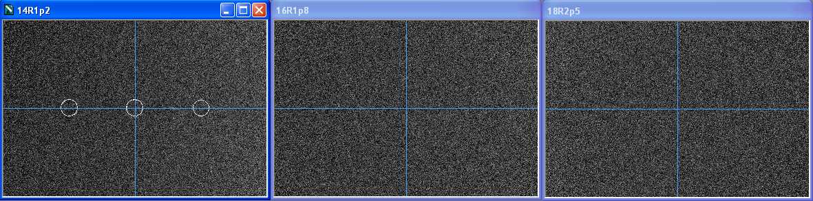
Figure 2. Result of flat-frame calibrating
even-numbered flat frame images using odd-numbered flat frames for
creating the flat from correction image (2004.10.08) showing excellent
removal of vignetting effects that require several % flat frame
corrections. The first frame shows where readings were taken.
Hardware/Software
Considerations: Context for
Remaining Tips
The remaining tips are somewhat hardware and software related. So
let
me state what I'm using and each observer can modify their procedures
to fit the hardware and software to be used.
I have a Celestron 14-inch (CGE-1400) Schmidt-Cassegrain telescope.
Given that for the IL Aqr observations require a large FOV in order to
include several reference stars on the main chip I employ a prime focus
configuration which many Celestrons are capable of (they call this
feature Fastar). My prime focus transition lens (for coma reduction and
flat fielding) is Starizona's HyperStar, which affords a fast f-ratio
of 1.86. If you can't use a prime focus configuration then you may need
to use a focal reducer lens to achieve a large FOV (i.e., larger than 8 x 12 'arc,.and
preferably ~16 x 24 'arc).
My CCD camera is a SBIG ST-8XE (9-micron square pixel dimension) and
I use a SBIG CFW-8 filter
wheel with photometric filters. This configuration produces an image
scale of 2.81
"arc/pixel and the FOV is 72x48 arc. Since the "atmospheric seeing"
typically is 2.5 to 3.0 "arc (FWHM), the prime focus configuration
point-spread function is much larger than the "seeing" limitation; my
observed FWHM is ~7.5 "arc. The only time this FWHM changes is when I
fail to update the focus setting (using plots of focus setting versus
temperature, with lines plotted for each filter - since my photometric
filters are not parfocal at prime focus).
The telescope is located
in a sliding-roof shed 50 feet from my house, and it is controlled
using 100-foot buried conduit cables from my house office (separate
conduit for AC power and control cables). I use MaxIm DL 4.0 to control
the telescope pointing, CCD camera, filter wheel and wireless focuser.
I change
focus using a wireless product Starizona sells (called MicroTouch) that
connects to the
shaft of the mirror focus knob. The wireless device works fine for all
telescope orientations, and it is supported by MaxIm DL.
For pointing I must use MaxPoint, a Cyanogen Ltd. product that is
similar to TPoint (TPoint can't be used with MaxIm DL but MaxPoint was
sritten by the MaxIm DL people so they work great together). MaxPoint
overcomes the bugs that afflict some of Celestron's CGE-series mounts
that render them incapable of reliable pointing). Since the darned
CGE's have to be flipped when crossing the meridian I have MaxPoint
coefficient files for the eastern half of the sky and the western
half of the sky. The appropriate MaxPoint coefficient file has to be
loaded before observing begins.
Observing
Procedure
A typical
observing night starts with observing schedule planning before an early
dinner. Tranist ingress and egress times dictate the start and end
times. It is absolutely necessary to allow for a set of sky flat frames
that begin at sunset and end 1/2 hour later (for my f-ratio). My use of
a "Double T-shirt Cover" for zenith sunset exposures is described
above. All dark
frame images (for each filter, if more than one filter was used) are
then averaged. The CCD cooler is
then set to a value that can be sustained (about -18 C at this time of
the year at my site). During CCD cool down I check telescope
pointing and verify focus on a star in the region of interest.
Observations of the exoplanet are preceded by another focus check
and a
star field position placement that provides a suitably bright star on
the autoguider chip. The
exoplanet is almost always placed at the center of
the FOV since with the prime focus configuration the autoguider chip
almost always has suitably bright stars present. My goal is to maintain
this placement of the star field with respect to the main chip for the
entire duration of the night's exoplanet observations. This is an
important
observing goal since errors in the flat field are an important source
of systematic changes in exoplanet brightness. Exposure times for the
exoplanet images are kept short enough so that none of the reference
stars
are saturated (maximum counts below 40,000). For TrES-1 and R-band this
exposure time could be as high as 60 seconds for my system, but so far
I have used only 30-second exposures.
When focus and pointing have been checked it's time to start the
autoguider. I try to keep a post-it record on the monitor showing
whether the last autoguider calibration was for one side of the
meridian or the other. This is useful for German equatorial mount users
since a meridian flip requires a "flip" box to be checked on the
autoguider set-up menu when observing on the other side of the meridian
from when calibration was done. Once the autoguider is running it's
good practice to monitor the small autoguider image window for awhile
to make sure the autoguiding is working right. Once autoguiding seems
to be working I take a deep breath and start the long series of
sequence observations. The hope is that the autoguider will not "get
lost" and drive the telescope far away, which would require a
time-wasting re-pointing procedure. If this happens, the main loss is
time coverage, not target star magnitude offsets related to use of a
slightly different part of the flat frame for reference and target
star. I have shown that with my system in the prime focus configuration
re-positionings that are 5% of the FOV different do not have any
noticeable effect on the target star's magnitude solutions. This might
not be the case for Cassegrain focus, where the flat field has more
structure.
I use MaxIm DL's "sequence"
observing feature to take many sets of 10 "light" images and one "dark"
image. My focusing is not automated, so I monitor FWHM "on the fly" by
quickly calibrating a sequence image while another is being exposed. If
the FWHM trend convinces me that a focus adjustment is needed the
sequence can be halted and a focus adjustment can be made manually.
It's important to not waste time with elaborate focusing procedure
while monitoring an exoplanet, so it's important to "know thy
instrument" and ake good estiamtes of what focus adjsutment is likely
to be needed (based on temperature).
I'm a firm believer in using an Observing Log with a ball-point pen.
Obseving log notations should never be capable of erasure, as they may
be invaluable when trying to reconstruct what happened at a later date
when memopry has faded. All post-observation notations on the Observing
Log should bemade in pencil. My OL is probably more meticulous than
most observers are willing to do, but that's the philosophy I
developed from several decades of field observations in a related field
before my retirement. For each observing sequence I note the UT start
time, sequence number, filter, exposure time, whether there's
autoguiding or not, focus setting, telescope tube temperature, outside
ambient temperature, wind seepd and direction. During the sequence I
note FWHM from "on the fly" readings of an unsaturated star while
another exposure is in progress. Every telescope pointing change for
re-centering is noted, as are the new indicated coordinates. At the end
of the night's observing I note my subjective impressions of how well
things went that night (whether goals were met, lessons learned, etc).
Data Reduction
My data reduction procedureis not automated, and I don't use a second
computer with a LAN to perform reduction analyses during an observing
session. Therefore, what I shall now describe may seem painfully
"primitive." The concepts of what I do are probably more sound
than my procedure for implementing them, so bear with me.
I use MaxIm DL's Photometry Tool
for photometric analysis of groups of images. I manually load 5 images
at a time, calibrate them (flat field and dark), and save the median
combined (or sigma-clip combine) image. I am very wary of cosmic ray
effects creeping into light curve analyses, so I always use median
combined (or sigma-clip combined) images for my photometric analyses.
After several groups of 5 raw/calibrated images have been processed to
produce "clean" images I perform a photometric solution for several
clean images using the MaxIm DL Photometric Tool. The exoplanet
"object" is chosen, and several "reference stars" are also chosen and
their magnitudes are entered in to the Photometric Tool. The choice of
signal aperture radius, gap width and sky reference annulus width are
important, and for the prime focus configuration I usually use 5, 2 and
4 pixels. The stars typically have FHWM = 2.7 pixels, so use of 5
pixels for the aperture radius is "conservative" in the sense that for
images when the FWHM is larger than for other images there will be
minimal effect on the "intensity" reading. Occasionally a star field
has interfering stars near a reference star and
this requires a different choice for aperture/gap/sky reference. Here's
a rule that should never be violated: Thou
shalt not use different signal aperture size for different images!
Absolutely all images of the exoplanet should be processed using the
same signal aperture radius, gap annulus width and sky reference
annulus width. The
Photometric tool creates a CSV-file containing a Julian Day time tag
and magnitudes for the object and reference stars.
There's a slight adjustment that is needed for the time tags when using
MaxIm DL Photometry Tool to create CSV-files. The time tag does not
correspond to the middle of all image exposures. I don't know why this
is so (should be easy to program), but every user should determine if a
time tag offset is needed. This is done by manually calculating
mid-exposure time and comparing with the time tag in the CSV-file (or
whatever file your image processing software createts).
These CSV-files are imported
to an Excel spreadsheet and processed in a straightforward manner.
Checks are usually performed to validate constancy of the reference
stars with respect to each other, which is another way of using these
stars for the role of "check stars." Outliers data is dealt with by
referring to the observing log (as when I sometimes change focus
setting during an exposure, a bad habit which I'll admit to trying).
Any unexplained outlier is subjected to Pierce's Criterion (1876),
which can be briefly summarized as "when a suspected outlier is X
standard deviations away from where an average trace predicts it to be,
where X is chosen to be appropriate to the number of observations,
REJECT the data and repeat the search for more outliers." Instead of
using an average trace you can use nearest neighbors to assess
population SE and reject data using the same concept in Pierce's
Criterion. I believe in averaging (after rejecting outliers), and
there's an art to appropriate averaging - which isn't worth belaboring
here.
Dealing With Interfering
Stars
There's one problem with using *119 that everyone should be aware
of. There's a faint star ~17 "arc to the NNE (pa = 327 degrees) of *119
(see figure, below). The faint star is 3.0 magnitudes fainter than *119
using a V-band filter. My photometry of *119 excluded the nearby faint
star by employing a technique that would horrify most observers; I used
a pixel editing feature to "remove" the faint star from the image
(using a copy of the original for the horrific deed), then performed
the photometry using that edited image. (I'm practised in this from my
faint asteroid light curve work, where an asteroid is always going near
faint stars during the course of an evenning's observing.) I didn't
have the option of changing the "aperture radius/gap annulus width/sky
reference annulus width" settings because doing that would render my
equation predicted magnitude (described in the next paragraph) unusable
for those changed settings. The way I recommend handling this faint
interfering star for exoplanet monitoring is to set the signal aperture
so that the faint star is entirely within or entirely outside the
signal aperture (and not withni the sky reference annulus). The effect
of completetly including the faint star within the signal aperture is
to merely introduce a slight offset in the exoplanet magnitudes, and
provided all images are reduced with the same aperture settings this
will not cause changes in the exoplanet light curve.
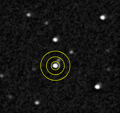
Figure 3. This is the preferred way to set aperture
radius, gap width and sky reference annulus so that the neaerby
interfering star does not affect the measured intensity of a reference
star. FOV = 6.0 x
5.8 'arc, north up, east left.
I suppose that I should mention that I employ a novel scheme for
converting measured star intensity to magnitude (described at http://brucegary.net/AllSky/x.htm).
It involves solving for coefficients in an equation that allows
extinction and star color. In my opinion it is simpler and superior to
the standard "CCD Transformation Equation" (derived and described in
all its gory detail at http://reductionism.net.seanic.net/CCD_TE/cte.html).
My all-sky procedure involves noting each reference star's "intensity"
(having units of "counts") and entering them in a spreadsheet. When the
user completes an iterative solution for two key coefficient values it
is possible to convert any star's intensity to an "equation predicted
magnitude." When this is done for the Landolt reference stars (of known
true magnitude) it is possible to compute an RMS difference between
equation predicted and true magnitude for the Landolt stars. This
method of assessing RMS accuracy can be used to predict the accuracy of
equation predicted magnitudes of any other star for which an intensity
has been measured. Based on the RMS scatter of the 14 Landolt star
magnitudes used for deriving the IL Aqr reference star magnitudes I
conclude that the B- and V-magnitudes listed in the table above have an
SE uncertainty of 0.033 and 0.022 magnitude. The B-V entries are
therefore subject to an SE uncertainty of 0.040 magnitude.
Data Analysis
Data analysis is what you do after data reduction. That's where real
thinking and real fun begins. For example, data analysis would include
1) deciding whether extinction that affected reference stars
differently
than the exoplanet star could have produced a trend versus air mass, 2)
deciding whether it's appropriate to average one transit data set with
another, and 3) modeling the effect of the transiting planet's size in
an attempt to determine the star's limb darkening.
Non-Transit
"Wander" Observations
To satisfy my curiosity about how big instrumental "wander" features
can be for my system I observed TrES-1 for 3.4 hours on a
non-transit night (2004.11.04) to see what level of variations would be
observed
using the same observing hardware configuration, observing technique
and the same data reduction procedure that was used for the transit
observations. Here are those observations for TrES-1 and a nearby
check star with approximately the same brightnesss.
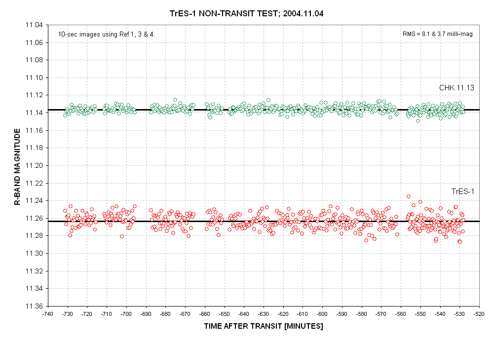
Figure 4. Measured R-magnitudes on a non-tranist
night for TrES-1 (red) and a check star
(green) using same hardware and procedures as during the transit
nights. Three stars served as reference ("comp").
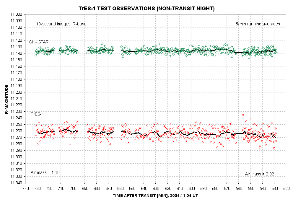
Figure 5. Light curve plot of same data as in
previous figure. A 5-minute
running average is shown.
The observations began with air mass = 1.10 and ended when airmass =
2.32. The RMS deviations from the running average increase with air
mass from 3.07 to 3.84 milli-magnitude for the check star and they
increase from 6.85 to 8.58 milli-magnitude for TrES-1.
TrES-1 exhibits an RMS variation about the 5-minute running average
trace that is greater than for the check star. For example, at low air
mass the two RMS values are 3.07 milli-magnitude (check star) and 6.85
milli-magnitude (TrES-1). The RMS fluctuations are in the ratio 2.22
instead of the expected 1.12 (based on brightness ratios). I don't
understand this.
The 5-minute average trace for the check star exhibits a range of
variation of ~6 milli-magnitude, whereas the range of variation for
TrES-1 is about 10 milli-magnitude. Clearly, for my transit
observations features similar to those in the above figure should not
be believed. Specifically, a 5-minute feature with an amplitude of 2
milli-magnitude is too subtle for me to detect with one observing
session (especially when TrES-1 is at a high air mass).
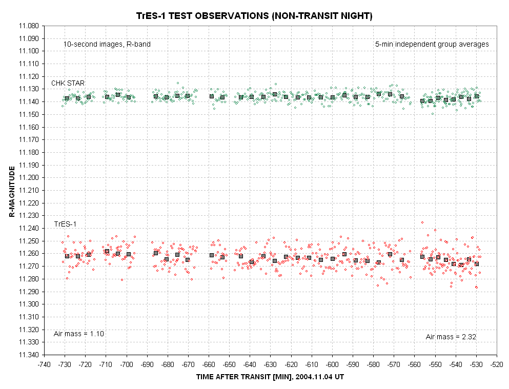
Figure 6. Light curve plot of same data as in
previous two figures. 5-minute
independent group averages are shown.
The 5-minute group averages for the check star exhibit an RMS about
their ensemble average of 0.88 milli-magnitude at low air mass to 1.56
milli-magnitude at high air mass. For TrES-1 the RMS deviations from
the ensemble group average is 2.25 milli-magnitude at low air mass and
2.42 milli-magnitude at high air mass.
The check star 5-minute independent group average of 0.88
milli-magnitude at low air mass agrees well with the value expected
from the 10-second individual image RMS of 3.07 milli-magnitude (0.89
milli-magnitude). The check star's high air mass RMS is slightly higher
than the expected value, 1.56 versus 1.11 milli-magnitude. I interpret
this to be evidence that high air mass observing conditions produce
systematic errors that wander by amounts greater than the stochastic
uncertainty (for my system). This appears evident in the check star's 4
milli-magnitude "fade feature" at about -575 to -555 minutes. TrES-1's
5-minute independent group averages undergo a greater fluctuation than
the check star, as predicted from their greater RMS for individual
10-second images. The TrES-1 5-minute groups exhhibit approximately the
expected RMS values for both low and high air mass, being 2.25 versus
2.00 milli-magnitude for low air mass and 2.42 versus 2.48
milli-magnitude for high air mass.
Using the 5-minute independent data groups it is possible to predict
the level of features that can be expected to appear during a real
transit event, assuming stochastic SE and systematic wander
characteristics are the same both observing nights. TrES-1 and the
check star tell the "same story": we should expect to see non-real
10-minute features with amplitudes ~2 milli-magnitude at low air mass
and ~3 milli-magnitude at high air mass. Given the better stochastic
behavior of the check star (than TrES-1) these systematic error
wanderings will be more apparent for a star that is stochastically
well-behaved (like the check star was). For a star with poorer
stochastic behavior (like TrES-1) the systematic error wandering will
be less apparent (although it is approximately the same as for the
stochastically well-behaved check star).
Another way to approach the question of whether to believe features in
an exoplanet light curve is to perform a transit simulation using
non-transit observations. This is done in the next two figures.
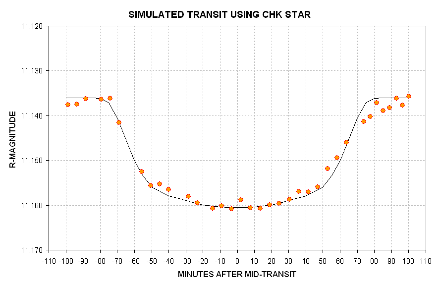
Figure 7. Simulated light curve using measurements
of a nearby check star and adjusting them using a hypothetical transit
light curve with TrES-1 properties.
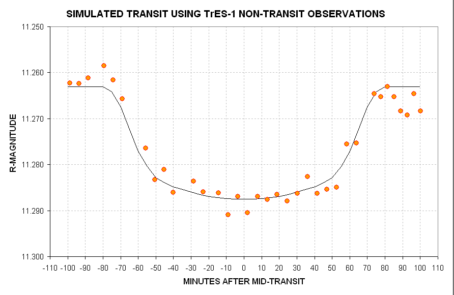
Figure 8. Simulated transit light curve using TrES-1
non-transit observations and adjusting them using a hyothetical transit
light curve with TrES-1 properties.
The two figures, above, were created from the non-transit measurements
of 2004.11.04 by applying a hypothetical transit light curve shape
adjustment to the non-transit observations. These plots show what can
be expected when observing a transit. If the "eye" detects features in
these light curves then the "brain" should intervene and say "no,
they're not real; they're roduced by systematic error wander." Indeed,
in the second of these simulated transits (based on TrES-1 non-transit
observations) note the apparent "bump" before ingress. There is no
corresponding brightness bump after egress, and in fact there appearsto
be a fading after egress. The first of these "features" must be
attributed to systematic error wander and the latter feature may be due
to wander associated with high air mass.
The "message" from this simulation is that instrumental anomalies
having amplitudes of ~3 or 4 milli-magnitude should be expected from an
observing system (and analysis procedure) used by the author of this
web page. If other observers want to argue for the "reality" of their
anomalies then it may be instructive for them to conduct a simulation
using non-transit observations similar to what I have described on this
web page. As an alternative light curves obtained by several observers
could be combined to see if all of them, or most of them, show the same
anomalies. That analysis will be performed for the TrES-1 2004
October/November observations by Aaron Price (AAVSO) in the near
future.
In the above two figures notice the better "behavior" of the check star
compared with TrES-1. As stated earlier, I do not undersxstand why
TrES-1 has a higher
stochastic SE than the check star (whose brightness is only 12%
greater). It may have something to do with nearby faint stars with PSFs
whose edgtes wander in and out of the signal aperture or sky reference
annulus. Or maybe the three reference stars were better located for
removing flat field errors (i.e., the reference stars "surrounded" the
check star better than TrES-1).
This exercise illlustrates some of the considerations and supporting
observations that can lead to improved understanding and performance in
exoplanet transit monitoring.
Results
for TrES-1
The following results were obtained for exoplanet TrES-1during October,
2004.
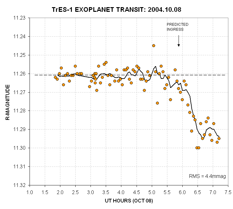
Figure 9. Each datum is from a median combine of
five 30-second exposures, and represents an observation taken within a
200-second observing window (which allows for image download time). A
photometric R-band filter was used. The first observations were made
just after transit and the observations end when the elevation was 19
degrees (m=3.1). Two "outliers" occur (near 5.0 hours) when I was
negligently changing the focus setting. The residuals from an average
trace have an RMS = 0.0038 magnitude (excluding the two "outliers").
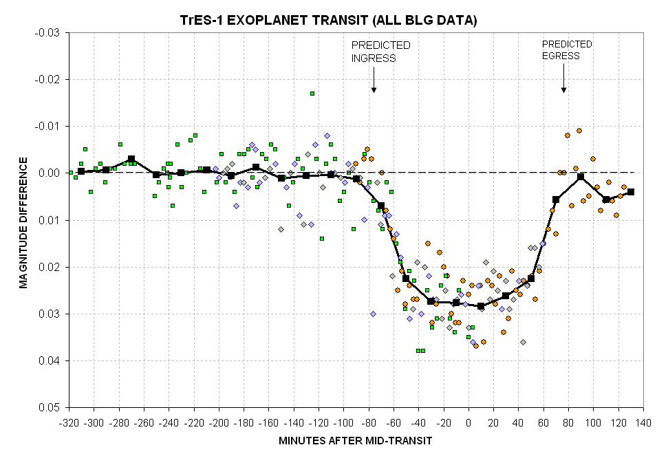
Figure 10. All data from three transit observing
sessions are combined in this graph. The average trace is for 20-minute
chunks
of data. The vertical offsets were subjectively chosen. I estimate that the 20-minute averageshave a
precision that ranges from ~1.8 millimagnitude for most of the
pre-ingress data to less than that for the mid-transit section.
Miscellaneous
Links
Artificial Star Photometry
XO-1 observations
AAVSO home web page is at http://www.aavso.org/
AAVSO CCD observer's manual is at http://www.aavso.org/observing/programs/ccd/manual/
My TrES-1 observations of three transits is at http://brucegary.net/TrES-1/x.htm
My HD209458 observations of one transit (in 2002) is at http://reductionism.net.seanic.net/HD209458/ExoPlanet.html
AL Aqr (GJ 876) reference
stars
My general interest AstroPhotos web page with many links is at http://reductionism.net.seanic.net/brucelgary/AstroPhotos/x.htm
My observatory in Hereford, AZ is shown at http://reductionism.net.seanic.net/brucelgary/AstroPhotos/m_hardware.htm
and you can reach me at the following e-mail address: b r u c e g a r y 1 @ c i s - b r o a d b a n d . c o m

____________________________________________________________________
This site opened: October 11,
2004. Last Update: June 25,
2007