Collisions as the Source for
White Dwarf Transiting Dust Clouds
Bruce L. Gary, Last Updated
2021.06.10
This web page
addresses a poorly understood aspect of how collision
dust clouds work.
Introduction
There are three known white dwarfs
(WDs) with transiting dust clouds. For two of them the dust
clouds appear to be in circular orbits: WD 1145+017 and
J0328. The discovery paper for the first of these proposed
that the dust clouds were produced by sublimating minerals.
This was a reasonable suggestion since the temperature of
the planetesimal associated with the dust clouds was
extremely hot, due to its closeness to the WD. Shortcomings
slowly accumulated for this dust production mechanism, and
with the discovery of dust clouds orbiting the latest
discovered WD there is additional concern that sublimation
may not be the cause for dust clouds orbiting WDs. This is
because at a distance where the J0328 asteroid source is
orbiting temperatures are too cool for minerals to sublimate
and too hot for volatiles associated with comets. There
should therefore be new interest in the collision model as
an alternative for generating dust clouds. This web page
addresses a poorly understood aspect of how
collision-generated dust clouds work.
Links Withing this Web Page
Celestial
mechanics
Dust
cloud shape evolution
Debris disk and parent fragment
Specific collision case study
Interesting
properties of dust clouds produced by a collision
Observational
evidence
Conclusions
Further reading
References
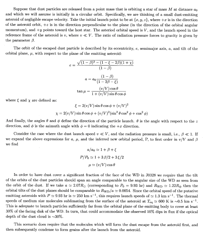
1. Celestial Mechanics -
Vertical Motion
Let's begin with an imaginary "explosion" of a rock in orbit just
above Earth's equator. Before the explosion the rock was traveling
with velocity V oriented parallel to the equator. Consider
a particle that undergoes a delta-V during the explosion in the
upward direction (i.e., parallel to the rotational axis). It is in
a new orbit determined by it's trajectory following the explosion.
This orbit will be inclined by angle alpha = atan (delta-V / V).
It's ground track will be just like satellite tracks that we've
all seen:
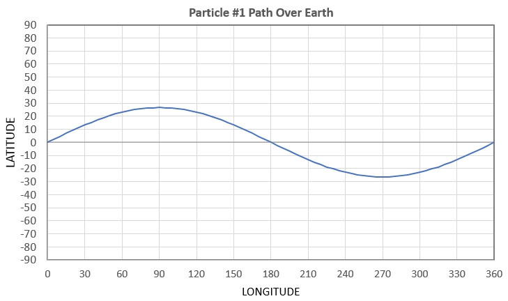
Figure 1a. Path over earth of particle #1 if delta-V = ½×
V.
Now consider a particle with delta-V of the same magnitude but
oriented in the opposite direction:
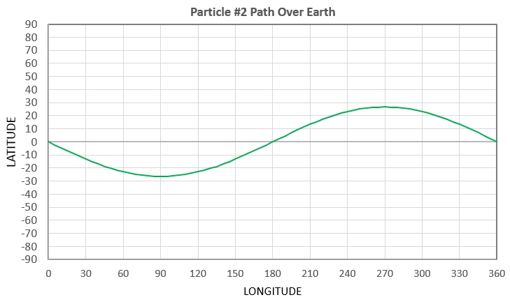
Figure 1b. Path over earth of particle #2 if delta-V = -
½× V.
Here's the path of both particles:
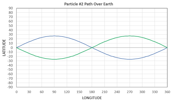
Figure 1c. Path over earth of particles #1 & #2 if
delta-V = ± ½× V.
Notice that the two particles start out going away from each
other, reaching maximum separation 1/4 orbit later, then come
together at the opposite longitude of the collision, followed by
another separation and coming together back at the original
explosion site.
An explosion will have many particles with a range of delta-V.
Here's what a few particles could do:
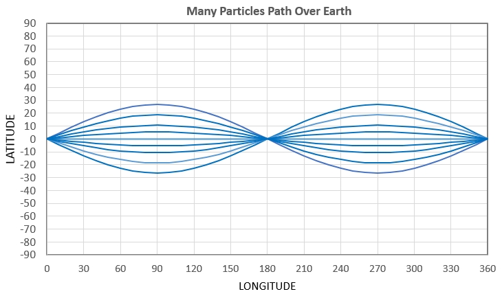
Figure 1d. Path over earth of many particles from same
explosion.
The cloud of particles can be described as expanding and
contracting twice per orbit. For this example the maximum
size of the cloud is ~ ½× RadiusEarth. The properties of
different size clouds (different delta-V max) will be the same.
Celestial Mechanics - horizontal Motions
Let's change terminology and use the term "collision" instead of
explosion; this is appropriate since both produce ejecta in all
directions (isotropic). Let's also shift to the site of a WD,
instead of the Earth. A collision will produce delta-V in other
directions than up and down. Radial components will produce
eccentric orbits. They will have the same orbital period since no
angular momentum was lost or gained by these inward/outward
components. Here's an example of new orbits caused by inward and
outward delta-V, using the WD1145 case for illustration. The view
is from above a pole, looking down on the orbit plane.
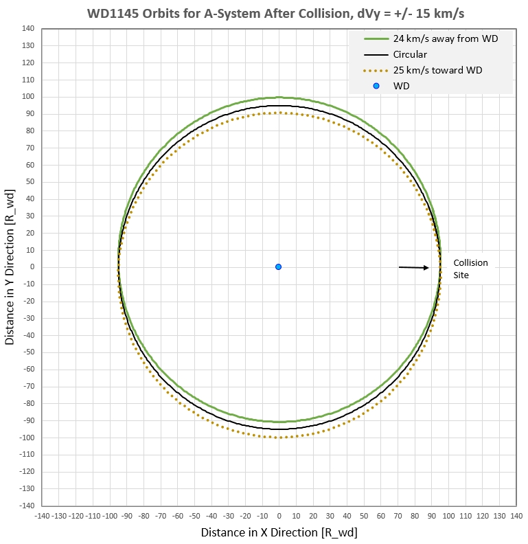
Figure 2a. Orbits for ejection in direction
perpendicular to orbital motion, inward (toward the central
object) and outward, assuming delta-V = 24 km/s (exaggerated for
illustration purposes from a more realistic 1.5 km/s).
Ejected debris expands and contracts twice per orbit.
The forward and aft components will produce eccentric orbits with
different periods, since angular momentum is gained and lost by
these delta-V components. This is illustrated in the next diagram
(using WD1145 for illustration).
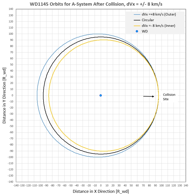
Figure 2b. Pole view of orbits for ejection in
direction of orbital motion (forward and backward) assuming
delta-V = +/- 8 km/s (exaggerated for illustration
purposes from a more realistic 1.5 km/s). Ejected debris
expands and contracts only once per orbit. Since periods
differ the debris in different orbits won't return to the
collision site at the same time; this will produce dust cloud
smearing along the orbit.
Initially, after the explosion, the dust cloud will expand to
maximum size after 1/4 orbit, then collapse to a small oblong (long
in the radial direction) at the opposite longitude, followed by
another expansion and contraction, ending back at the collision site
as a tiny cloud of particles with their original velocities.
The previous two diagrams exaggerate the differences in orbits
because they are used to illustrate a concept. Here are two
counterpart diagrams that are realistic since I've adopted maximum
speeds of 1.5 km/s.
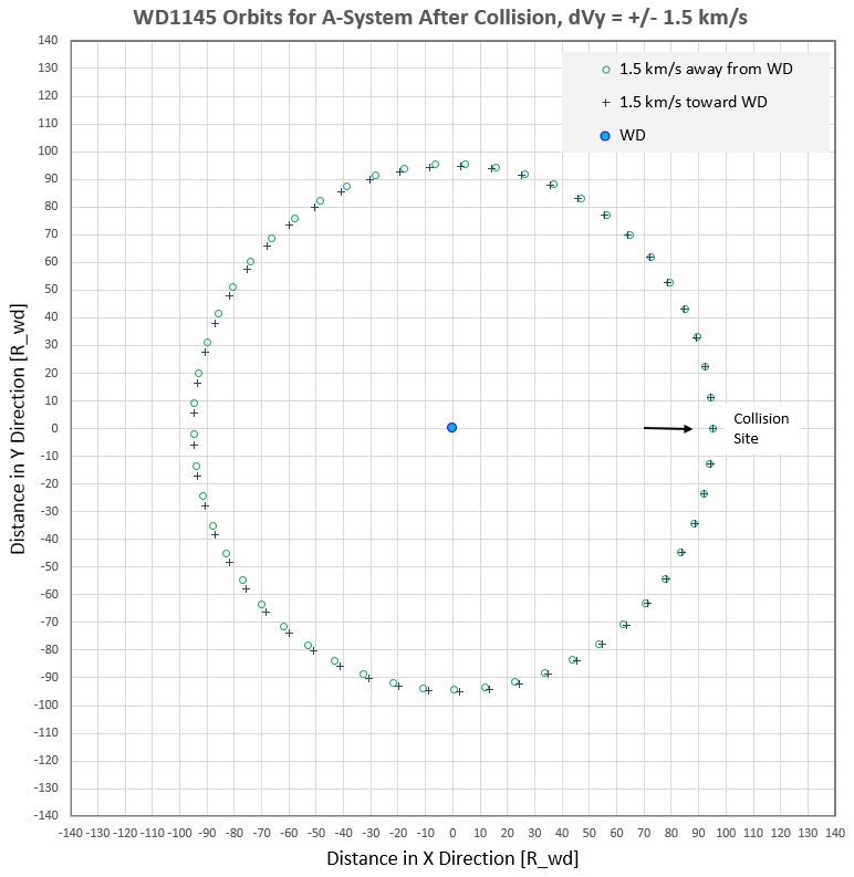
Figure 2c. Locations are shown at 5-minute intervals for
orbits of particles ejected in radial directions toward and away
from the WD. A sense of the cloud length can be seen by the
separation of corresponding points. For example, the cloud is
spread out the most on the left side, opposite the collision
location. The periods are the same since no orbital momentum
changes are involved.
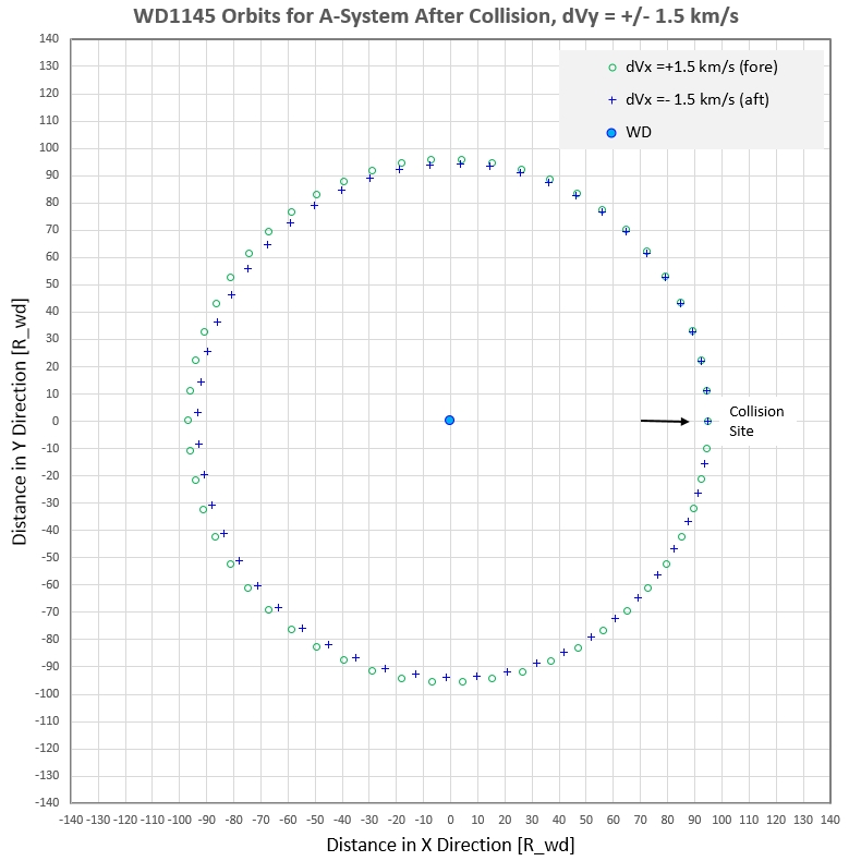
Figure 2d. Locations of particles ejected parallel to
orbital motion with delta-V = 1.5 km/s, shown at 5-minute
intervals. The periods differ, and the particles arrive back at
the collision location at different times. The "aft-ejected"
particles begin to go ahead of the "fore-ejected" particles at ~
1/4 orbit. At the half-orbit region the aft lead is ~ 5 minutes.
By the end of an orbit the aft particle lead is ~ 8 minutes.
The previous two figures show how different the sizes vary with
orbital phase for particles ejected parallel to orbital motion and
parallel to the radial direction. This causes dust cloud stretching
that is episodic for one direction and accumulative for another. The
next figure illustrates this.
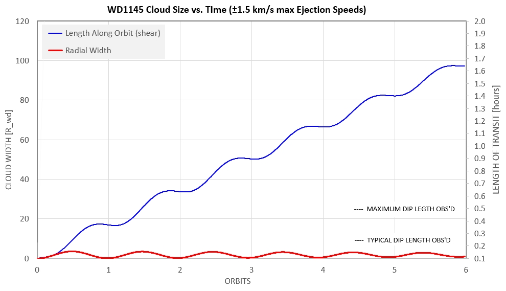
Figure 2e. Size of dust cloud in the orbital plane vs.
time for an adopted 1.5 km/s maximum ejection speeds. The blue
trace shows stretching along the orbit ("orbit shear") that
increases approximately monotonically. The red trace shows size
variations in the radial direction, which is sinusoidal and
confined to 3.6 R_wd (diameter), or ± 1.8 R_wd with respect to a
circular orbit. The scale on the right is in units of dip length,
from ingress to egress.
Dips are never observed to be longer than ~ 30 minutes long (ingress
to egress), so something must be removing particles before ~ 1.5
orbits. Usually, this removal occurs during the first 1/2 orbit.
This is one of the WD1145 mysteries!
One answer to the "orbit shear" mystery that is tempting to consider
is to adopt ejection speeds lower than 1.8 km/s. However, we need
these high speeds to account for observed dip depths. These speeds
cause vertical displacements (see Fig. 1d) that reach WD latitudes
of 20 to 40 degrees. Optically thick dust clouds that are stretched
out along the orbit by several WD radii have to be this large in
latitudinal expanse in order to produce the observed dip depths of
30 to 60 %.
3. Dust Cloud Shape
Evolution for 400 m/s Maximum Injection Velocities
The following sequence of figures show dust cloud size and shape vs.
time for a full orbit. It is assumed that dust is ejected
"isotropically" (within the orbit plane) with maximum speeds of 400
m/s. This is a 2-D model; particle motion perpendicular to the orbit
plane is not modeled. The source for particles is orbiting
counter-clockwise. All views are looking down (pole view).
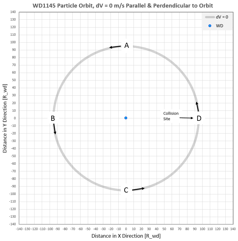
Figure 3a. This orbit was obtained by placing a test
particle at x,y location +95.1, 0.0 (Rwd units), specifying a
velocity component in the upward direction of 315.17 km/s and zero
component in the horizontal (radial) direction. The central star
is WD1145 and was assigned mass = 1.19e30 kg. At equal time
increments of 3 seconds acceleration was calculated and the
associated velocity increment vector was added to the previous
time step velocity to obtain a new velocity vector. Small
adjustments of the initial velocity were made in order to achieve
a circular orbit.
Vertical displacement versus orbit phase in shown n the next graph:
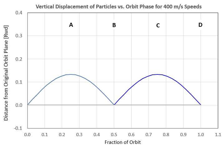
Figure 3b. Vertical displacement of 400 m/s particles vs.
orbit phase. The phases A, B, C and D correspond to orbit
locations in the previous figure.
The displacements in the orbit plane, in x.,y coordinates, was
modeled by specifying an initial x,y location and assigning delta-V
components of 400 m/s in the 4 cardinal directions (up, left, down
and right). The following sequence shows the location of these 4
particles at times corresponding to 1/4 orbit locations (referenced
in the above figure as locations A, B, C and D). Location D is a
full orbit after the simulated "collision." The 4 particle locations
for each 1/4 orbit interval define an ellipse within which all
slower moving particles should be found. The ellipses expand and
contract, change shape and rotate counter-clockwise. In the
following sequence the orbit motion is always to the left, and the
WD is always in the down direction.
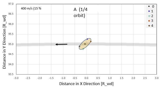
Figure 3c. At this orbit location, A, the cloud of
particles define an ellipse with maximum length ~ 0.5 Rwd and
oriented at 45 degrees with respect to the orbit (and rotating in
the counter-clockwise direction).
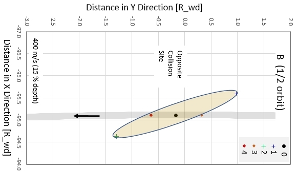
Figure 3d. At this orbit location, B, the cloud of
particles define an ellipse with maximum length ~ 2.4 Rwd that is
oriented at almost parallel to the orbit (and continues to rotate
in the counter-clockwise direction).
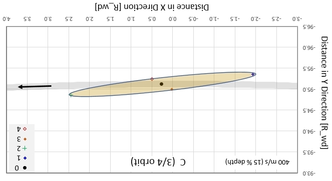
Figure 3e. At orbit location C the cloud defines an
ellipse with maximum length ~ 4.5 Rwd and is oriented at almost
parallel to the orbit.
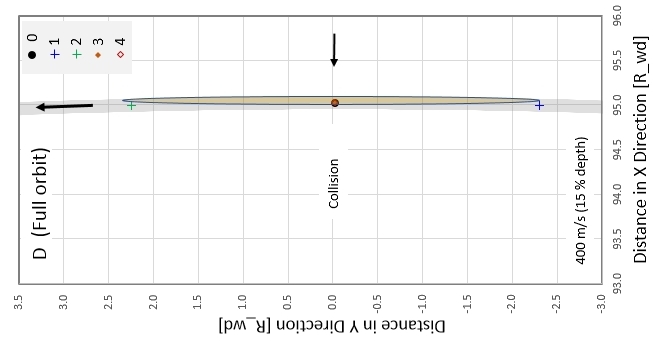
Figure 3f. At orbit location D, after one full orbit, the
cloud of particles define an ellipse with maximum length ~ 4.5 Rwd
that is oriented exactly parallel to the orbit. (The ellipse width
is actually much narrower than depicted.)
This sequence shows more clearly that Particle 1, for example,
is always farther from the WD than the source. It also is lagging
the other particles when the dust cloud completes an orbit by
returning to the collision location. These behaviors make sense
because Particle 1 was ejected in the forward direction, so it went
into a larger orbit, with a longer period.
It should be noted that during the orbit depicted above, there were
particles not included in this model that were ejected in the up and
down directions (perpendicular to the orbit plane), referred to as
motion in the z coordinate. Their distances from the orbit plane
underwent two cycles of expansion and contraction. For example,
assuming 400 m/s ejection speeds away from the orbit plane, at the
time depicted by "A" the z location was ~ 1030 km, or 0.12 × Rwd.
This corresponds to a blockage 15 % of WD light (assuming delta-V
occurs in both directions, and dust cloud is stretched out to at
least a WD diameter). Clearly, greater values for delta-V are
required.
The diagrams above (with maximum ejection speeds of 400 m/s) is
apparently typical for WD1145, because 15 % dip depths are common.
However, greater ejection speeds are needed to account for the
deeper dips. We need to consider maximum ejection speeds of > 1
km/s in order to account for observed dip depths as large as 65 %.
Maximum Ejection Velocity of 1.8 km/s
The next graph shows the relation between ejection speed and dip
depth. It assumes that the dust cloud is stretched along the orbit
many times Rwd, forming a horizontal band that passes through disk
center.
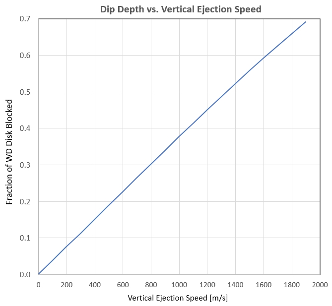
Figure 3g. WD disk blockage vs. ejection speed, assuming
an optically thick dust cloud that is greatly stretched by "orbit
shear" (i.e., broad band along orbit).
Since dips have been observed with depths of 65 % we have to
assume that ejection speeds can be as large as 1.8 km/s. Sublimation
models are thought to be limited to a feww 100 m/s maximum speeds.
That's the main reason collisions are attractive.
4 - After Many Orbits
As shown in Fig. 2e the "along orbit size" of the dust cloud
continues to lengthen after the first orbit. After 6 orbits the dust
cloud is 100 R_wd in length. The circumference of the orbit is 600
R_wd, so the two ends of the dust cloud will come together after ~
36 orbits, or one week!
A more detailed calculation of orbits for particles ejected
isotropically has been performed by Jackson et al. (2014). Here's a
graph from that paper showing a parameter related to particle
density (projected onto the equatorial plane) after so many orbits
that a steady-state of particle density is achieved.
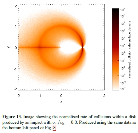
Figure 4. A figure from Jackson et al. (2014) showing a
parameter related to density of particles after many orbits of an
isotropic ejection of particles from a single collision.The
original collision site is on the right.
According to the above graph by Jackson et al. (2014) the greatest
probability of additional collisions after the initial one is
located at the original collision site. Note that after a
steady-state is established (when "orbit shear" no longer changes
the shape of where debris is found) the debris disk has a volume
that is fixed in inertial space. The thickness of the debris disk is
maximum at the 1/4 and 3/4 orbit azimuths e.g., one R_wd), and
thickness is very small at the collision and opposite azimuth. The
minimum of thickness at the 1/2 orbit azimuth produces a high
density of debris and accounts the line of high probability of
collision in the above figure.
All the preceding description is for a single collision that
produces an isotropic ejection of particles that spread out to form
an asymmetric debris disk. We are now ready to consider one crucial
new aspect of the model: what if the original fragment survives the
original collision and continues to orbit within the debris disk?
Fate of a Large Fragment that Produces a Debris Disk
Imagine that a large fragment is impacted by a smaller fragment and
this produces isotropic ejection of particles that form a debris
disk (after a week or two, assuming, for now, that we're dealing
with WD1145). The debris disk will have a "particle size
distribution" (PSD) that ranges from photometrically relevant (<
1 micron radius) to photometrically irrelevant (>> 1 micron)
yet collisionally relevant. There is a finite probability for
additional collisions during each passage of the parent fragment
through the high density region of the debris disk original
collision site. This probability is specified by the density of
particles, the PSD function and the size of the parent fragment. If
this probability is close to one, then during every orbit the parent
fragment will create a new component of debris that starts out small
and undergoes the expansion pattern described in the previous
sections. In this way the original debris disk is continually added
to, or at least replenished. Since the new component of debris
begins confined to a small volume it may have a sufficient density
of photometrically relevant particles to be optically thick. The
debris disk, on the other hand, is so spread out that a
line-of-sight through it at a random azimuth may be optically thin.
Note that particles >> 1 micron are relevant for producing
collisions, but are unimportant for blocking light (simply because
they are much less numerous).
Keep in mind that the debris disk is a volume with a specific shape,
fixed in space, with debris whizzing around at km/s speeds, and the
parent fragment is orbiting within it and encountering debris with a
density that varies with the same pattern during each orbit. There
will in fact be several fragments orbiting within this debris disk.
Over time, as the cascade of secondary collisions accumulate, the
parent fragment will lose mass and shrink. With a reduced size it
will be less likely to encounter debris, so the dust cloud that is
kept in place around it will dissipate and it will no longer produce
dips.
Consider the scenario in which the original collision yields several
large fragments in similar orbits. After a debris disk is
established from that collision (after a week or so) each large
fragment will experience collisions within the debris disk where
debris density is the greatest (site of the original collision), and
each of these secondary collisions will contribute to replenishing
the debris disk. If several fragments are in similar orbits they can
all experience greater activity becasue they all pass through the
debris disk's high density region. In this way one fragment's
increase in activity can cause neighboring fragments to also
increase their activity. This was observed in 2017 for WD1145 (see
Fig. 7h, below).
This is a mechanism that might be capable of maintaining an
optically thick dust cloud with a stable dip depth and width until
the fragment loses mass and shrinks in size so that it no longer has
a high encounter probability. What's needed for assessing the merits
of this model are detailed calculations showing quantitatively that
encounter probabilities are high enough to sustain the steady-state
replenishment of a parent fragment's fresh and small-sized debris
clouds with sufficient optical depth to produce dips similar to
those that are observed.
5 - Specific Case Study
Let's try to "quantify" a collision scenario that could account for
some of the observed dip behavior. Some of my assumptions will
surely need revision since I'm not expert on collisions. My purpose
for this exercise is to show that a collision model can work if a
large volume of N-dimensional parameter space is allowed for
exploration. It will up to others, more knowledgeable on collisions
and sublimation, to determine whether or not a feasible volume of
this parameter space can account for observed dip behavior. My
excuse for entering this unfamiliar territory is that no one else is
doing it, and someone should start doing it!
I'll start with the following assumptions:
1) the parent fragment is 10 km in radius
orbiting in a 4.5-hour circular orbit around WD1145,
2) an initial collision occurs when a 1 km object
(0.1 % as massive) impacts the 10 km object which produces debris
from the completely shattered smaller object
(debris from the parent object will also be included in the debris
cloud but it will not be considered in this case study),
3) this initial collision produces debris with a
size distribution of large chunks (i.e., < 500 m radius),
4) subsequent collisions (a "cascade") populates
smaller sizes, down to 0.3 micron eventually,
5) debris has a velocity distribution that is
isotropic and has a maximum speed of 500 m/s,
6) the smallest particles have the highest
speeds,
7) the fragment and debris cloud is observed from
Earth to cross the WD disk at an orbit location 3.7 hours past the
collision site,
8) sublimation occurs for particles smaller than
1 micron radius
For these assumptions Earth observers see the dust cloud when it is
at an orbit position 252 degrees of azimuth past the collision site
(between B and C in Fig. 3a). The vertical extent of the cloud is 78
% of its maximum extent, and provided the cloud is broader in
azimuth than the WD, an opaque cloud would produce a dip depth of 14
%. This is the median depth observed during the first 3.5 years of
ground-based observations (which explains the specifics of some of
the above assumptions). I am not assuming that the cloud is opaque
on the first orbit; more things have to happen to produce a high
opacity. Here's the extent of the cloud 3.7 hours after the initial
collision.
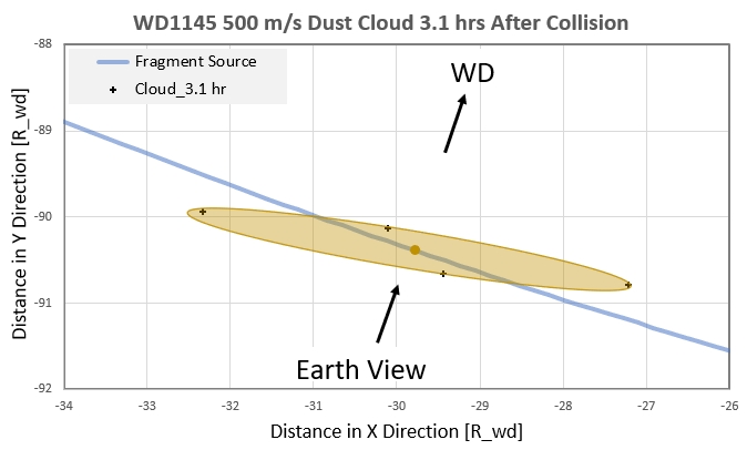
Figure 5a. Extent of dust cloud 3.1 hours after the
initial collision.
Keep in mind that the above figure shows the extent of the smallest
particles. Large particles, which I will refer to as debris, will be
confined to smaller volumes. Since its the small particles that
dominate optical depth (e.g., < 5 micron radius), any dip that is
produced by this cloud will have a length (ingress to egress)
corresponding to the outer limits of the dust cloud, which for the
above case would be 5 x R_wd / 300 km/s = 9 minutes (assuming high
opacity throughout the cloud). So far, all these cloud properties
are compatible with dip observations.
Let's estimate the optical depth of the the dust cloud at the
3.1-hour time of its evolution. To do this we have to adopt a
"particle size distribution" (PSD) function. Instead of using an
analytic model, since this is just a demonstration of approximate
feasibility, I'll treat particles as belonging to one of 10 size
bins, as illustrated in the next figure.
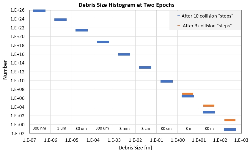
Figure 5b. Debris radius histogram after 3 and 10
collision "steps."
In this PSD model it is assumed that we begin with one object with a
radius of 1000 m at time step 0. A time step interval is defined to
be how long it takes for half the number of objects in a size bin to
be converted to the next smaller size bin. Therefore, during the
collision cascade each size bin loses objects to the next smaller
bin and gains a smaller number of objects from the next larger bin
(if objects are present there). The log/log slope of the
steady-state histogram is close to that observed for Saturn's
A-ring: N(r) = c × r-11/4. As cascades continue the
right end of the function decreases, meaning that the original 1 km
object eventually is worn down to nothing - which eventually happens
to the large chunks created by the initial impact.
This oversimplified model has the unrealistic assumption that one
collision produces only fragments in the next smaller size bin. In
reality, a fraction of a second after an initial impact faster
moving fragments will be colliding with slower ones, so in fact one
impact unleashes a cascade of smaller collisions as the debris
leaves the initial impact site. Therefore, all size bins can be
populated after the initial impact. The procedure used to create the
above histogram is just a mathematically convenient way to determine
the shape of a histogram after some form of steady-state is
achieved, which might happen after just the initial impact.
After the cascade of collisions has led to a steady-state (all size
bins populated and the largest size bin is still populated) it is
possible to calculate the projected area of all particles. This is
shown in the next graph: This figure illustrates why the smallest
particles dominate blockage of WD starlight.
.jpg)
Figure 5c. Projected area of all particles in specific
size bins, assuming no overlap.
The most important size bin is 3 microns, which has a projected area
for all particles in that bin = 2e13 m^2. For comparison, the
projected area of a WD1145 hemisphere = 11e13 m^2. The sum of
projected area for the 3 micron, 30 micron and 300 micron bins
(particles within the size region 1 micron to 1 mm) equals 3.8e13
m^2. This is sufficient for producing a 35 % depth dip (if there was
no overlap of particle areas). It is conceivable that when
considering particle overlap a 14 % dip could be produced by the
scenario under consideration. Notice that all debris larger than ~ 1
mm is irrelevant for producing dips. Their projected area (for this
model) is a mere 9.4e11 m^2 (or < 1 % of WD1145 hemisphere).
You'll notice that I omitted inclusion of the 300 nm particles in my
calculation of projected area for the dust cloud. This is because
these small particles have been shown to rapidly overheat and
sublimate out of existence (Xu et al., 2017).
At the time corresponding to Fig. 5a, after less than one orbit
following the original collision, according to this model the PSD
will consist of only large debris; i.e., no debris as small as 0.3
micron. Therefore, this model predicts no dip depth for the first
orbit through the Earth's line-of-sight (LOS) to the WD. A more
realistic model would produce some debris at all sizes, but probably
very small amounts at 0.3 micron, meaning that during the first
orbit following an initial collision there should not be an
observable dip.
Assumption 6, above, states that only the smallest particles have
velocities as great as 500 m/s. I have no idea how to model the
function for collision ejection speed vs. particle size, so I've
decided to consider the possibilities shown in the following figure:
.jpg)
Figure 5d. Arbitrarily selected functions describing
ejection speed vs. particle size, using the equation V =
constant / (radius ^ exponent).
Note that if all particles had the same kinetic energy the speed of
30 m chunks would be an astoundingly low 1e-7 m/s (assuming 500 m/s
for 1 micron particles), so I reject this assumption for guidance in
adopting a model for velocity vs. particle size. Since particles are
colliding with each other after the initial impact there will be an
effective "viscosity" which will cause faster particles to lose
speed and slower particles to gain speed. I have no idea how to
model this situation, and maybe the best way to learn about this is
from laboratory experiments. Since I'm not aware of the results of
such experiments I will adopt an arbitrary model. A first step is to
adopt one speed for each particle size. This overlooks the more
realistic case in which each particle size exhibits a histogram for
speed (e.g., Maxwell-Boltzmann distribution, or something similar).
The above chart is intuitively reasonable and I have adopted the
middle model (exponent = 0.2). Accordingly, during the debris
cloud's first passage through the Earth's LOS most of the debris
won't be as spread out as shown in Fig. 5a. For example, the 30 m
chunks will be moving with a speed of ~ 30 m/s whereas the 1 micron
particles will be moving with speeds of 500 m/s. This means that the
large chunks will have a rate of expanding along the orbit ("azimuth
shear") that is only ~ 6 % of that for the 1 micron particles. This
is important because it means we can account for the presence of
dips that don't change their width or depth for weeks by viewing the
large chunks as continuously producing small particles which have a
finite lifetime, as will be discussed below.
Referring back to the histogram of debris size (Fig. 5c), after a
steady-state is established half the mass of the debris cloud will
be in chunks with a size greater than 3 cm, traveling with speeds
less than 60 m/s. This population of large debris can be viewed as a
source for future dust particle production. The following figure
shows how confined in space this large debris population is.
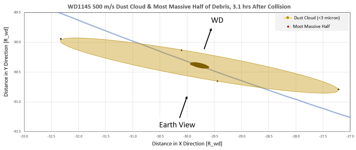
Figure 5e. Extent of small particle dust cloud (< 3
micron) and most massive half of debris (> 3 cm), 3.1 hours
after the initial impact.
It's possible that during the dust cloud's first passage through the
Earth's LOS, 3.1 hours after the collision, there could be a
sufficient number of small particles to produce an observable dip.
If so, then the shape of the dip would be determined by the velocity
distribution versus particle size. Let's predict what our simple
model so far predicts for optical depth versus distance from the
large (10 km) fragment. So far my model assigns just one speed for
each size bin. This exercise will therefore provide a way (in
theory) to derive a speed histogram vs. size. One candidate for a
speed function is the Maxwell-Boltzmann distribution, shown below:
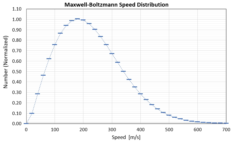
Figure 5f. A Maxwell-Boltzmann distribution histogram for
speeds with a "tail" near 500 m/s (corresponding to 3 micron
particles in the above model).
For larger particles their speeds will be slower, as shown in
the next graph:
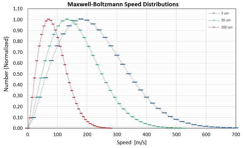
Figure 5g. Maxwell-Boltzmann distribution histogram of
speeds for particle sizes 300, 30 and 3 micron (assuming the
relation in Fig. 5d).
Consider the fact that the number of 3 micron particles is ~ 250
times the number of 30 micron particles (in Fig. 5b). Another way to
illustrate this big difference is shown in the next figure.
.jpg)
Figure 5h. Speed histogram for 3 particle size bins.
Since a particle in one size bin obstructs 100 times the area of a
particle in the next lower size bin the importance of particles
versus size is better portrayed in the next graph.
.jpg)
Figure 5i. Total area blocked by particles per increment
of speed, for three size bins.
As already noted, in terms of blocking WD starlight the 3 micron
particles (size range of 1.0 to 10 microns) are the most important,
with less importance for each larger size bin. But what's the number
density of particles versus distance from the 1 km asteroid that's
near the center of the dust cloud after a specific time, such as 3.1
hours after the collision? If we begin with an assumption of
spherical symmetry (no Keplerian azimuth shear) this is easily
calculated by assuming that particles are distributed in a series of
concentric shells whose radii are set by the speed of the inner and
outer boundaries for the size bin under consideration. For example,
at time t seconds after the collision the shell containing 3 micron
particles traveling at 100 m/s extends from radii = t × 90 m/s to t
× 110 m/s. The density of particles in that shell is simply the
total number of particles in that size bin and within that speed
range (Fig. 5h) divided by the volume of the shell (4 × pi × r2
× delta-r). The light blocking power of this subset of particles is
obtained by multiplying 1) the number density by 2) the
cross-section of each particle by 3) the projected area of the
volume cell under consideration. Figure 5i is a convenient
combination of parameters that can be used for this task.
It will be helpful to calculate, for each size bin, particle number
density vs. radial distance from the center (e.g., from the parent
asteroid, with radius 10 km). This will entail calculating shell
radii boundaries (using Fig. 5h), which determines the shell's
volume. Knowing the total number of particles within this volume
enables calculation of particle number density within that shell.
This is the particle number density that we seek.
.jpg)
Figure 5j. Number density vs. radial distance from the
large asteroid at the center of the debris cloud, for 3 size bins.
What we really need is the projected area of the particles per cubic
meter vs. radial distance from center. This is shown in the next
graph.
2.jpg)
Figure 5k. Projected area of particles in a cubic meter
vs. radial distance from center, for 3 size bins.
Finally, here's the sum of projected area, per cubic meter, for the
3 size bins we've considered vs. radial distance from the cloud
center.
3.jpg)
Figure 5l. Projected area per cubic meter of the three
size bins added together vs. radial distance form the center.
With this knowledge we can now consider a way to create a light
curve dip for a hypothetical observer who sees the above-described
cloud pass through his line-of-sight. We shall perform this
calculation using a cube of cells that includes the spherical dust
cloud at t =3.1 hours. For each cell, with x,y,z coordinates, we
calculate distance from the center, which allows for a determination
of the projected area of the three particle sizes (by simply
multiplying the value from the above figure times the volume of the
cell).
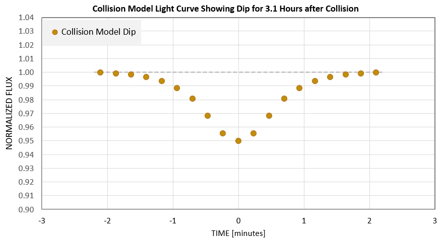
Figure 5m. Shape of light curve dip for the above modeled
dust cloud, using size bins: 3, 30 & 300 microns.
Question: We know that essentially all observed WD1145 dips can be
fit by an "asymmetric hypersecant" (AHS) function, so can the model
dip be fit by an AHS function?
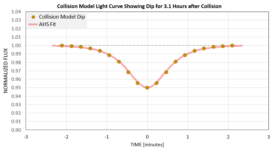
Figure 5n. Asymmetric hypersecant (AHS) function fit to
the model dust cloud dip.
The answer is "Yes, the model dust cloud's predicted dip shape can
be fit by the AHS function!"
The collision model predicts a very short dip length when the cloud
is observed only 3.1 hours after the original collision. Whereas total
dip length is ~ 4 minutes the FWHM length is 1.2 minutes. If this
dust cloud had been observed somewhat later, at the 3.65-hour time
after the original collision (same vertical extent), the FWHM dip
length would have been 1.5 minutes. Such short dips are rare but
they have been observed when large aperture telescopes with high SNR
have been used (e.g., Croll et al., 2017, Gaensicke et al., 2016). I
conclude that original collision events are capable of producing a
mature, or steady-state distribution of particle sizes. In other
words, it is possible to observe a dust cloud during its first orbit
following a collision. However, most observed dips are broader and
require more than one orbit to produce the typical 5 or 10 minute
FWHM lengths. This topic will be addressed below.
So far we've seen that a collision with the adopted assumptions can
produce a dip that resembles some observed dips after less than an
orbit following the original collision. The model assumption that
makes this possible is that during the original collision there are
a sufficient number of secondary collisions (during the seconds
following the original collision) to populates all bin sizes in a
way that resembles a steady-state.
The next goal is to assess the feasibility of the 10 km fragment
undergoing secondary collisions every time it passes through the
original collision site; I will refer to this location as "the
funnel."
Here's the view of the dust cloud after exactly one orbit, when the
parent fragment and all debris has returned to the original
collision site.
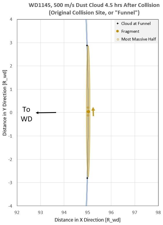
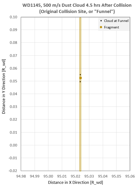
Figure 5p. Two views of extent of small particle dust
cloud (< 3 micron) and most massive half of debris (> 3 cm),
4.5 hours after the initial impact (when the 10 km parent asteroid
fragment and all debris returns to the original collision site
after just one orbit). In the left panel the width of the dust
cloud is greatly exaggerated. The small arrow pointed up has a
length corresponding to the extent of the most massive half of
debris. In the right panel, which is a90-times magnification of
the left panel, the length along the orbit of the most massive
half of debris extends well beyond the graph borders (+/- 0.2
R_wd). In both panels the parent 10 km asteroid fragment is
represented by a circular symbol.
The radial width of the dust cloud edge is very small, e.g., 0.00034
R_wd (2.8 km) for the crude calculation of this analysis (time-steps
of 5 seconds). Theoretically it should be zero, and it would have
been if the accuracy of my celestial mechanics had been perfect.
However, this zero width assumes that there were no secondary
collisions during the seconds following the original collision. I
haven't been able to include these secondary collisions in this
model so the width at the funnel will have to be assigned arbitrary
values. For example, if the last of these secondary collisions
occurred 1 second after the original collision then the loci of
orbit origins for all particles will be confined to a sphere 500 m
in radius, and this would determine the width of the dust cloud at
the funnel location.
Let's think of the funnel as a section of a ring of length 4 R_wd
with a circular cross-section having a radius that is somewhere
within the range 100 m to 4 km. Prior to the dust cloud's arrival at
the funnel particles will be "collapsing" toward the funnel ring
(i.e., orbit) with speeds the same as they left the original
collision site one orbit earlier. At some specific time before
reaching the original collision site we can imagine a snapshot of
the locations and velocities of the small and larger particles,
which is shown in ht next figure.
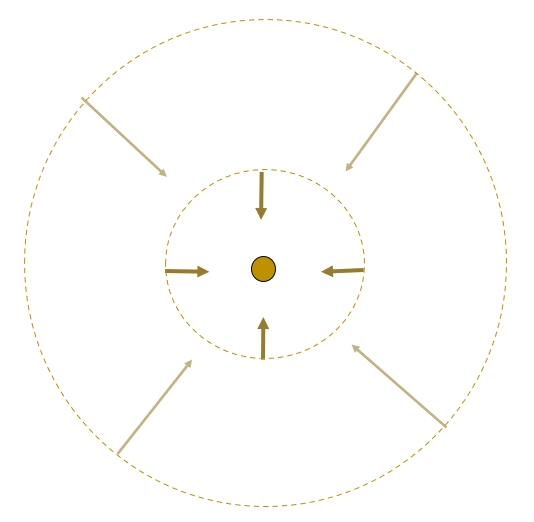
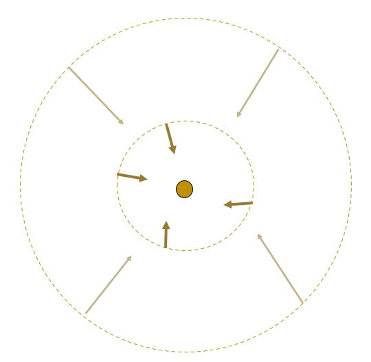
Figure 5q. Geometry of particles collapsing to original
collision site (where the 10 km fragment is located) showing how
the smallest particles are coming in from greater distances and at
greater speeds than the larger particles. Left panel shows what a
symmetric pattern of velocity vectors would look like, while right
panel shows velocity vectors that result from secondary collisions
concurring during the few seconds following the original
collision.
Keep in mind that these particles are collapsing like shrinking
tubes aligned with the orbit, and the parent fragment is located at
just one position along the tube's center line. In calculating the
probability of a collision of a particular particle with the 10 km
parent fragment this will be important.
In addition to collisions of particles with the parent fragment
there can be collisions of particles with each other. Both collision
types have to be considered when evaluating the ability of funnel
passages to replenish dust lost to sublimation during the previous
orbit. The easiest collision type to calculate is debris/parent
fragment, so that's waht I'll treat next.
Notice that the width of the dust cloud stated above, 500 m or less,
is much smaller than the size of the parent asteroid fragment of 10
km. This means we can assume that all particles will collide with
the 10 km parent fragment when the particles cross the orbit plane
when the 10 km parent fragment is at the same orbital azimuth. By
same orbital azimuth is meant same to within 10 km. For example,
consider the 3 micron particles. They cross the orbit plane when
they are stretched out along the orbit a distance of 5.5 R_wd
(diameter, using the 500 m/s particles for defining cloud size). A
particle density-weighted distance would be ~ 3 R_wd (total length),
or 1.5 R_wd (radius), which is 1.5 x 8.4e+6 m = 1.2e7 m. The 10 km
(radius) parent asteroid fragment represents a fraction of 1e-3 of
this cloud's length. In other words, only ~ 0.1 % of the 3 micron
particles collide with the 10 km parent fragment.
Using this approach for the other particle size bins yields the
following figure:
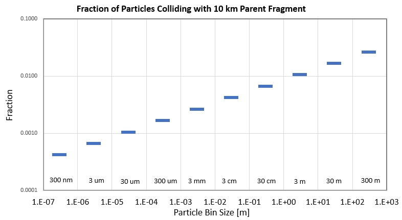
Figure 5r. Fraction of particles colliding with the 10 km
parent fragment after one orbit as a function of particle size.
About 3 % of the 300 m debris will collide with the 10 km parent
asteroid fragment after one orbit. These collisions will add to the
number of particles in the 30 m size bin. This is a small change,
and since the percentage additions for all other sizes are even less
impressive we can see that "particle/parent" collisions won't be an
important contributor to dust cloud longevity.
Next let's consider "particle/particle" collisions.
Temporary halt in this modeling project!

6 - Interesting Properties of
Collision-Created Dust Clouds
[This section needs revisions related to the insights described
in the previous section.]
A collision resembles an explosion. Ejected particle directions
will be approximately isotropic for both. The range of speeds will
have a maximum, and everything smaller should exist. A collision
in orbit will therefore be followed by the same behavior described
above.
Consider what might happen at the times of minimum size.
Particles (and larger fragments) are likely to collide, and could
produce a new population of smaller particles. A quasi-continuous
production of new particles may occur twice per orbit. A particle
size distribution will eventually be achieved. The total absorbing
and scattering power of the dust cloud at a given phase could
therefore vary: a steady decrease due to orbit shear plus
occasional injection of a new population of particles during the
contraction phases.
If particle injections are isotropic then some will be in shorter
period orbits and some will be in longer period orbits. These will
be the particles that had an ejection velocity component in the
forward or afterward directions. Because of there being a range of
periods for the particles the shape of the dust cloud will spread
out along the orbit more each orbit. The shape will evolve from
spherical shortly after the collision to an ellipsoid with a
circular cross-section. The length of the ellipsoid will increase
with time. I'll refer to this process as "orbit shear."
Observations of dips show the effect of orbit shear during the
course of a few days after a dust cloud forms. However, the
stretching out along the orbit reaches a maximum amount and the
length of the dip remains approximately constant for many more
orbits (weeks, o until the dip disappears). What can limit the
stretching caused by orbit shear? We don't know, but we can
speculate. I can think of two candidates for limiting orbit shear
stretching: 1) particles in smaller orbits (with periastrons
closer to the WD) will be hotter, and may sublimate. This could
limit the length of the ellipse in the forward direction
(ingress). 2) particles in larger orbits (apoastrons father from
the WD) will be in the way of dust clouds generated by the
planetesimal in the next farther out orbit. For example, WD1145's
inner-most planetesimal, in the "A" orbit, is at a distance from
the WD of 97.6 R_wd. The nearest neighbor planetesimal is in the
"D" orbit, at 98.4 R_wd. In the rotational reference frame of the
"A" system the "D" dust clouds are moving past the "A" dust clouds
in an outer orbit (in the backwards direction). Those "D" dust
clouds will be expanding and contracting, just like the "A" dust
clouds. Any "A" particles that venture out far enough may
encounter an expanded "D" dust cloud; when this happens it will
have its orbit altered due to impacts with "D" dust. Ironically,
the "D" dust will impart a forward delta-V to the "A" particle,
and cause it to be in an even larger and longer period orbit. In
the extreme case the "A" particle could be "entrained" by the "D"
dust cloud. This would remove it from the ellipsoidal "A" cloud,
and lead to a limit on how far in the aft direction (egress) the
ellipsoid could extend.
I haven't worked out numbers for the effects described in the
previous paragraph, so this is so far just speculation on why
orbit shear has a limit on how stretched out (along the orbit) a
dust cloud can become. Those effects are destructive, in the sense
that the "A" dust cloud is losing particles wthat had been ejected
with too great a component of forward or backward velocity
component. This particle loss of a dust cloud is compensated by
particle production that occurs at each compression cycle. The two
processes, particle loss rate and particle production rate, should
lead to a steady-state size for the ellipsoidal dust cloud. We
need such a result in order to be in agreement with observations
(next section).
Note that if the cloud is detected by its absorption and
scattering of light from a central source (a WD) the observer's
longitude will determine what phase the cloud is at each time it
transits the central object. The observer will see the cloud at
the same phase, every time, and won't know whether the cloud is
much larger or smaller for other hypothetical observers at other
longitudes.
A collision could produce gas as well as particles. The gas will
expand and contract synchronously with the cloud. The gas will
have a distribution of velocities along the line-of-sight, which
wil vary with phase. At the maximum expansion phase the
distribution of radial velocity will be close to zero width. The
distribution of velocities will be maximum when size is minimum.
If WD light is absorbed by the gas it is theoretically possible to
determine which phase is being observed. There will be an
ambiguity, of course, except at maximum and minimum phase when the
radial velocity spread is minimum and maximum, respectively.
Notice that the cloud's optical depth will vary in opposite
manner with size. The same cloud could be physically small and
optically thick for an observer at one longitude, and the opposite
for an observer at another longitude. Earth-based observers may
think that a shallow dip is for a small cloud, but we have no way
of knowing that the same cloud might be viewed by some alien
civilization as large with a deep dip depth.
If both gas and dust are present in a cloud the "viscosity" of
the cloud will vary with a cycle of half an orbit. Maximum
viscosity will occur when the cloud is smallest. This might
inhibit the effect of orbital shear by altering the velocities of
the particles with extreme relative velocities.
Dips that appear suddenly, with no evidence of any dip activity
prior to the start date, can be easily explained by this collision
model. A "turn-on" can occur whenever there's an impact of two
significantly massive chunks.
A collision might not create a dust cloud initially, but instead
create just two or more chunks that themselves can later become
the source for dust clouds. The daughter chunks will be in
different orbits, and will drift with different slopes in a
waterfall diagram. Each daughter chunk can have a different
"turn-on" time, depending on when other pieces in close orbit with
a neighbor chunk impacts the main chunk (during a minimum size
phase), or when other smaller pieces that accompany the main chunk
impact each other. For example, if two chunks are created from a
larger one due to a collision, there is a finite probability that
they will impact each other during compression phases. Eventually,
when the chunks impact, they will create a dust cloud that is
observed as a dip turn-on.
If collisions have a characteristic impact speed there will be a
characteristic profile of velocities for the fragments and
particles. The most interesting parameter for this scenario is the
maximum velocity of particles. This will determine how large the
dust cloud will be at each of its maximum expansion phases. If,
for example, the WD1145 delta-V maximum is 1 km/s, the maximum
size of the cloud will be 2700 km (radius). During the maximum
size phase such a dust cloud will be a sphere of radius 2700 km,
and after orbit shear has spread out the cloud in the orbit
direction it will be an oblong with a cross-section of 2700 km
radius and many times this in length. WD1145 has a diameter of
8550 km, so if the dust cloud crossed the center of the disk, and
if the dust cloud was optically thick throughout, the cloud could
cover as much as 35 % of the disk area and reduce starlight by the
same amount. Since we often see dips this deep the 1 km/s model is
appropriate to consider. This thought will be developed in the
next section.
7 - Observational Evidence
Is there evidence for collisions? Yes, and mostly it comes from
waterfall plots. Consider the following examples.
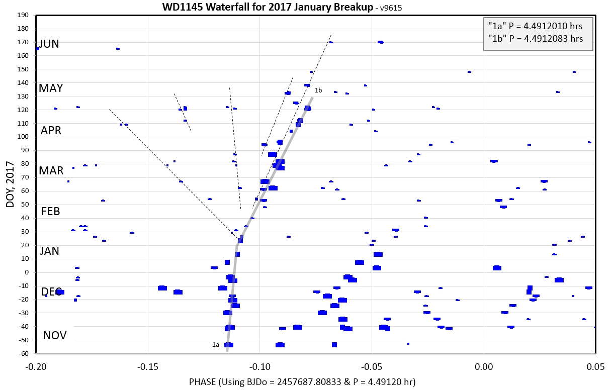
Figure 7a. An 8-month waterfall plot for WD1145 showing
one collision event with possibly 4 to 6 dust clouds following
different drift lines. Notice that "turn on" can take up to 80
days (420 orbits).
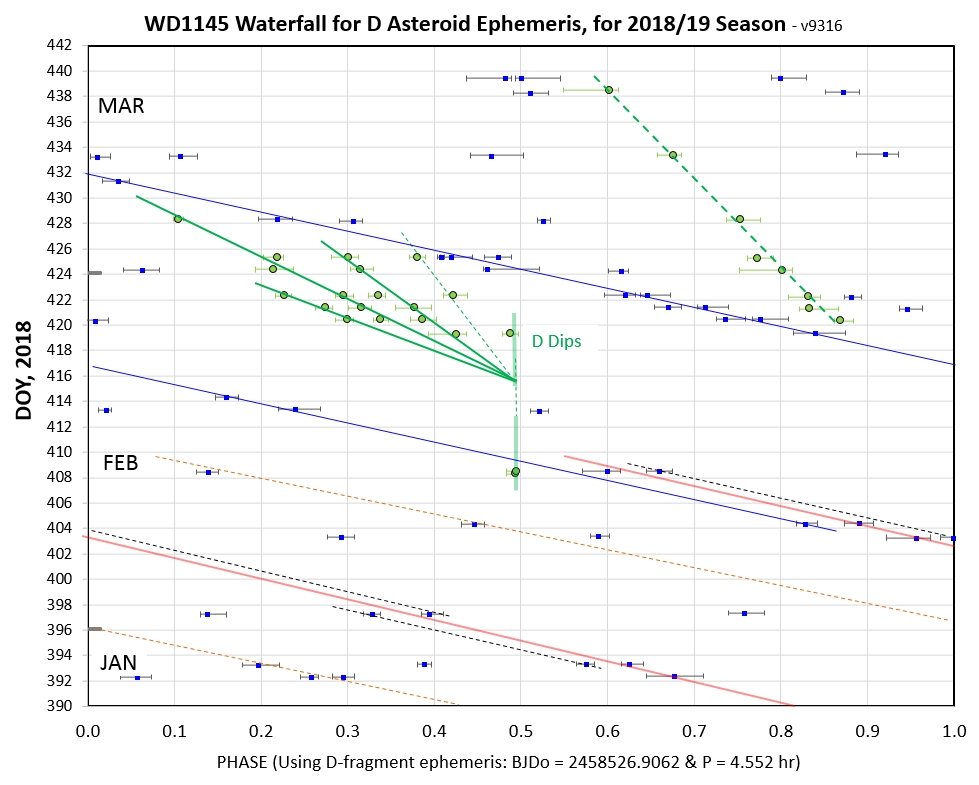
Figure 7b. A collision on Day 416 created 4 fragments
that "turned-on" 3 or 4 days later.
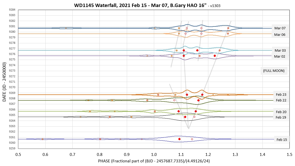
Figure 7c. Waterfall diagram suggesting that WD1145
underwent a collision event on 2021 Feb 17.
My last example of a collision found in a waterfall drift line
divergence pattern comes from the very first waterfall plot created
from ground-based observations (Rappaport et al. 2016).
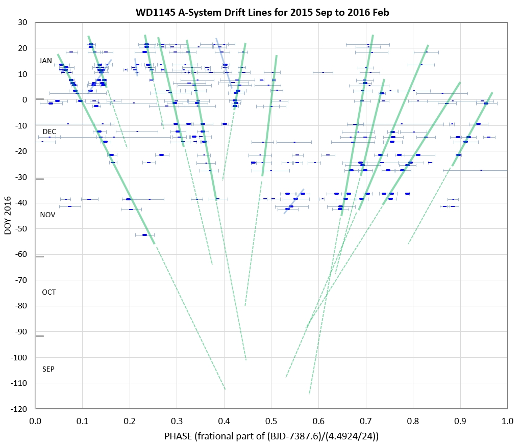
Figure 7d. These drift lines diverge from a date in
August, 2015, which corresponds to the time dip activity level for
WD1145 increased dramatically, by a 100-fold, compared with
ground-based measurements made 5 months earlier and before that by
the Kepler spacecraft.
An indirect way to check for consistency with collisions is to
compare histograms of dip depth with collision model predictions.
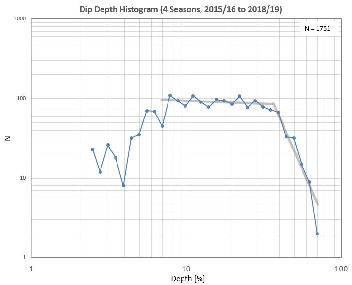
Figure 7e. Histogram
using uniform intervals for log(depth).
In the above
histogram depths < ~ 7 % are under-counted due to SNR
limitations of my telescope (14"). The break at 40 % is real
and may be related to the inclination of dust cloud orbits
that produce a preference for transiting in front of one
hemisphere of the WD disk more than the other hemisphere.It
could also be related to the maximum dust particle velocities
produced by collisions 9e.g., ~ 1.5 km/s). A
crude comparison of the observed flat slope is in agreement with a
model developed by Kenyon and Bromley. More work is needed on this
matter.
According to Kepler data WD1145 has dips with 6 different
periods, ranging from 4.5 to 4.9 hours. Consider the most active
period of 4.5 hours, which corresponds to a circular orbit radius
of 97.6 × R_wd. If dust clouds with a cross-section radius of 0.35
× R_wd are common (as derived in the previous section), and if
they are usually at the 97.6 × R_wd orbit location, they could
"scour," and keep clean, less frequent dust clouds throughout the
region 97.6 +/- 0.35 R_wd, or from 97.2 to 98.1 R_wd. In other
words, we should expect to find that dip periodicities have a
characteristic spacing that is defined by the typical maximum
collision velocity for planetesimals. The next figure is evidence
that supports this speculation.
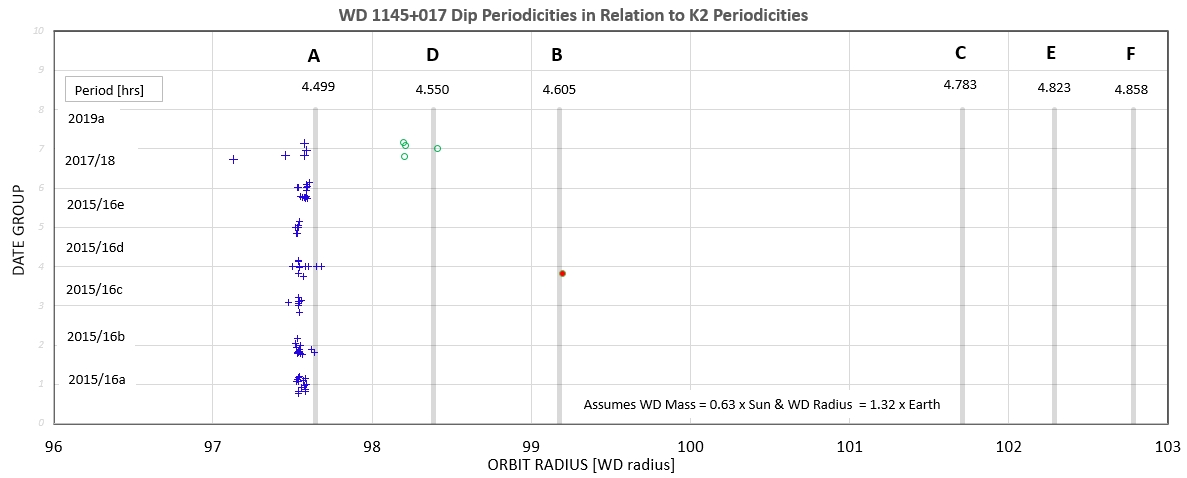
Figure 7f. The vertical lines correspond to the 6 Kepler
periodicities. Notice the approximately uniform spacing. (The
"missing" period corresponding to a distance of 100.5 R_wd may in
fact be present, but at a level undetected at the time of the
Kepler observations due to temporary inactivity.)
Based on the spacing it could be speculated that maximum
collision speeds are ~ 1.5 km/s. If the dust clouds produced by
these speeds are optically thick when they are at their maximum
size, then dip depths of ~ 60 % should occur (and they do).
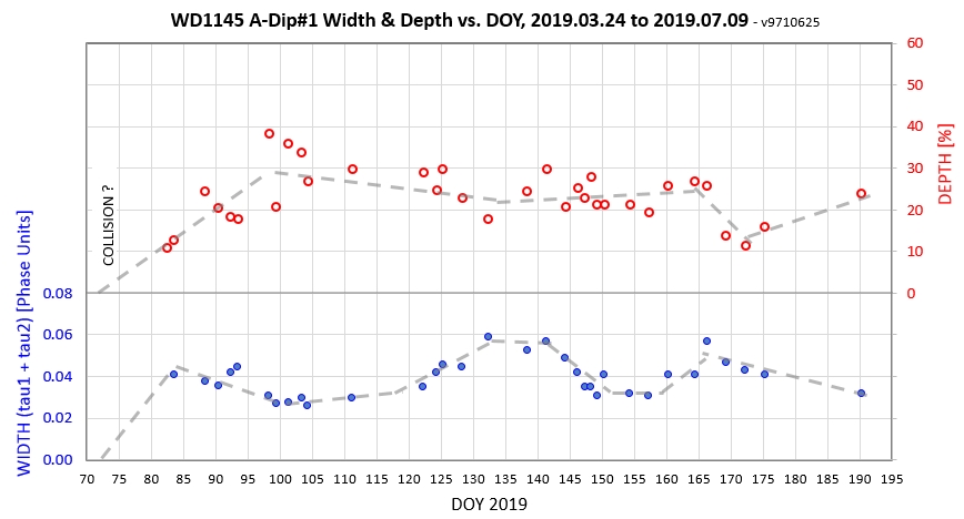
Figure 7g. Dust cloud width and depth vs. date
for a 3-month interval in 2019, for one specific dip.
This example may be what was described in the previous section
where orbit shear was discussed. Here's my scenario for events: 1)
An impact of two chunks in the "A" orbit occurred on about Day 72.
A spherical dust cloud rapidly expanded (during a 1/4 orbit) to a
size (and optical opacity spatial function) that obscured a few %
(<10 %) of WD light. The size of the cloud must have been
large, ~ 0.05 phase units (tau1 + tau2). This size corresponds to
~ 15 times the diameter of WD1145 (stretched out along the orbit
by "orbital shear"). 2) During each contraction (every 1/2 orbit)
the cascade of collisions continued and produced more dust in the
cloud. The optical depth of the cloud was increasing even while it
was decreasing in size. Why was it decreasing in size? Because the
particles with the farthest out apoastrons were entrained by the
"D" dust clouds, and were removed from the following edge of the
"A" ellipsoid" cloud. The leading edge may have been contracting
due to these particles orbiting closer to the WD and becoming hot
enough to sublimate. The cloud kept increasing in optical depth
until Day 100, when 30 % of WD light was blocked. 3) From Day 100
to the end of observations there was a steady-state production of
dust at minimum size times (when speeds and number density of
chunks were maximum) balanced by loss of particles to entrainment
by the "D" dust clouds and sublimation of the particles that
orbited too close to the WD.
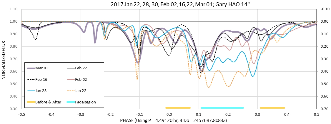
Figure 7h. An unusual case of a wide range of phases
undergoing simultaneous increases in activity, followed by a
coordinated decrease in activity.
Conclusion
Some evidence exists for collisions as a mechanism that produces
transiting dust clouds for WD1145.
Further Reading
Here's Saul Rappaport's derivation of equations to be used for
calculating key parameters for orbits of particles emitted from a
source that is in a circular orbit.
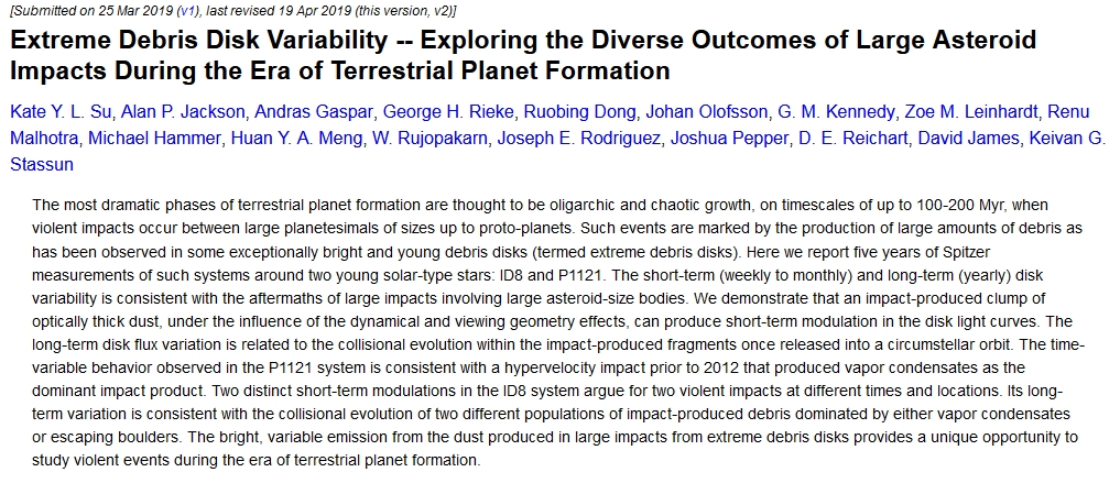
The planetary system formation community embraces collisions, as
exemplified in the following article:
This paper describes the celestial mechanics of the collection of
collision particles expanding and contracting twice per orbit (as
worked out by co-author Alan Jackson).
The arXiv preprint of this article is available at link
References
Jackson, Alan P., Mark C. Wyatt, Amy BOnsor and Dimitri Veras, 2014,
"Debris from Giant Impacts Between Planetary Embryos at Large
Orbital Radii," MNRAS, 440, 3757
Xu, S., S. Rappaport, R. van Lieshout & 35 others, 2017, "A
dearth of small particles in the transiting material around the
white dwarf WD 1145+017," MNRAS link,
preprint arXiv:
1711.06960
Croll, Bryce, Paul A. Dalba, Andrew Vandenburg and 12 others, 2017,
"Multiwavelength Transit Observations of the Candidate
Disintegrating Planetesimals Orbiting WD 1145+017," ApJ, 836:82 (pdf)
Gaensicke, B. T, A. Aungwerojwit, T. R. Marsh + 11 others, 2016,
"High-Speed Photometry of the Disintegrating Planetesimal at WD
1145+017: Evidence for Rapid Dynamical Evolution," arXiv 2015 link
____________________________________________________________________
This site opened March 06, 2021. Nothing on this
web page is copyrighted.