Fitting a Slope to X/Y
Measurements
Bruce L. Gary, Last Updated
2024.01.26
The task of solving for a
best-fitting slope for data with measured SE for both
the X and Y measurements can probably be performed by
adopting an average SE for the X and Y pair, allowing
for different SEs for different X/Y pairs.
Introduction
When Y is measured at a well-established X (such as time), the
probability isopleths for each measurement extend vertically above
and below the measured Y value in accordance with measurement
uncertainty, but they are essentially so narrow in the X direction
to warrant neglect. Most slope solutions are for such data sets.
However, when the X value is not something accurately determined
because it is another measurement with its own X uncertainty,
solving for a slope of Y vs. X is no longer straightforward.
Indeed, this problem is so infrequently encountered that it is
rarely described.
Equal SEs for X and Y
Consider the following data set of measured dip depth of white dwarf
J0328-1219 where one telescope measured dip depth using a g' band
filter and another telescope measured the same dip with a R band
filter. The g' and R depths are assigned to X and Y, respectively.
These data are shown in the first panel of the next figure.
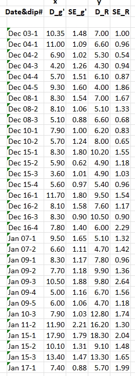
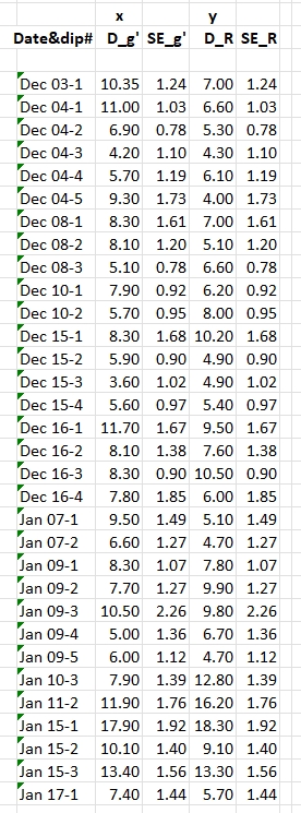
Figure 1. Left panel: measured g' and R band depths for
32 dips. Right panel: same depths but with SEs set to the average
of the g' and R measured SEs for each pairing.
A seen in the first panel, above, measured SEs for a pairing are
actually not equal. The second panel shows SEs that are equal, being
the average of the two measured SEs. As a first approximation we
will solve for a best fitting slope, with it's SE, using data in the
second panel. Later, I will assess the error for such a slope
solution by considering the impact of asopting equal SEs for each
pair.
In the next graph the first data point is shown with two of its
probability isopleths. The isopleths are circular because the SEs
for X and Y were set equal to the average SE for X and Y. A
candidate slope line is shown (with an assigned slope of 1). The
larger probability isopleth is the one that is tangent to the
candidate slope line. The distance between the data point and the
slope line is a distance labeled "d." The inner probability
isopleth, with a radius of "s" (1.24 units), corresponds to the SE
for Data #1.
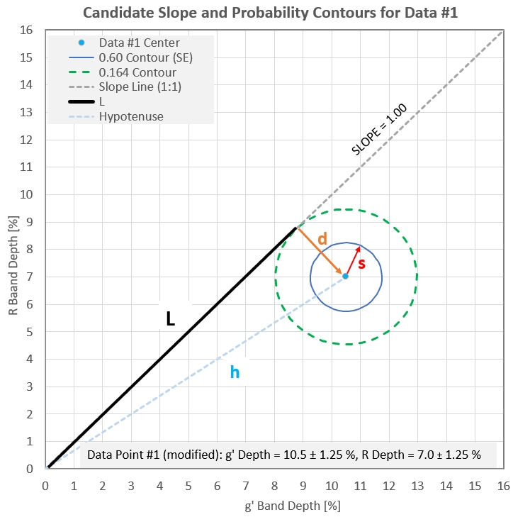
Figure 2. Scatter plot of g' and R measurement for Data
#1, showing probability isopleths for the SE (inner circle) and
the isopleth (outer circle) that is tangent yo a candidate slope.
For each candidate slope line we want to calculate the sum of
chi-squares for all 32 data measurements. For Data #1 the chi-square
is (d/s)^2. The length "d" is the hypotenuse of a small triangle
with a horizontal side having length = X - L × cosine (atan (f)),
where f = slope (expressed as a fraction; for this illustration f =
1.00). The vertical side has length = L × sine (atan (f)) - Y.
Calculating L is described in the next paragraph..
L is obtained by noting that sides "L":, "d" and "h" (from the
origin to Data #1) form a right triangle. The small angle of this
triangle at the origin can be obtained by subtracting the angle to
the slope line (atan f) and the angle to Data #1 (atan Y/X). Let's
call this small angle alpha. We can then invoke the rule that a /
sin(A) = b / sin (B) which allows us to evaluate d = h × sine
(alpha). Finally, L = sqrt (h^2 - d^2).
Once this procedure is implemented for Data #1, it can be repeated
for the calculation of Chi-Sqr_i = (d_i / s_i)^2 for i = 1 to 32,
yielding a sum-of-chi-squares (SCS) for the candidate slope. This
should be done for a selection of slope values in order to create a
plot of SCS(f).
Let's do this for the data in Fig. 1 (right panel).
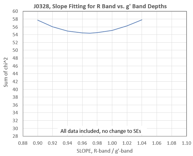
Figure 3. Sum of chi^2 for 32 measurements (using all
data and SEs as measured).
There are two things to notice about the above figure. First, a
solution for slope exists, and it's f = 0.97. Second, the lowest
"sum of chi squares" is greater than 31 (the number of measurements
minus the number of degrees of freedom, 32 -1). If we adopt the
model as being suitable for use with the data, we are forced to
assume that either all SEs are under-estimated or "outlier data" is
included in the analysis (and should be rejected). Data #2 has a
chi^2 = 8.1, while the median is 0.89 (for the best tentative
solution), so let's reject it.
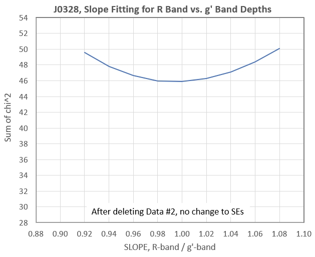
Figure 4. Sum of chi^2 for 31 measurements (one outlier
excluded, using SEs as measured).
There aer no more outliers in the 31 data set, so no more data
exclusions are permissible. The fact that the lowest "sum of chi
squaaares" is greater than 30 (N-1) means that the measured SEs are
under-estimated. This is not surprising given that there's a
subjective step in the process for measuring dip depth: setting the
out-of-transit level for each light curve. This step can lead to a
component of "systematic errors" quite distinct from the stochastic
situation upon which the SEs are based. We are allowed to adjust the
set of 31 measured SEs. Normally this is done by multiplying all SEs
by the same number. However, given that systematic errors may be
involved the manner for adjusting SEs might better be to
orthogonally add whatever amount brings the sum of chi squares down
to 30.
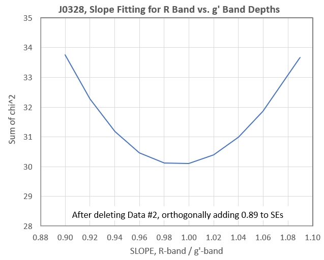
Figure 5. Sum of chi^2 for 31 measurements (one outlier
excluded, orthogonally adding 0.89 to measured SEs).
If the procedure to this point is valid, then we could state that
the best-fitting slope to the R and g' band measurements of dip
depth is:
Depth
ratios = 0.99 +/- 0.05
In other words, the J0328 dust clouds that produce dips are Mie
scatterers because all relevant dust particles are large compared to
optical wavelengths.Here's a scatter plot with this best-fitting
result:
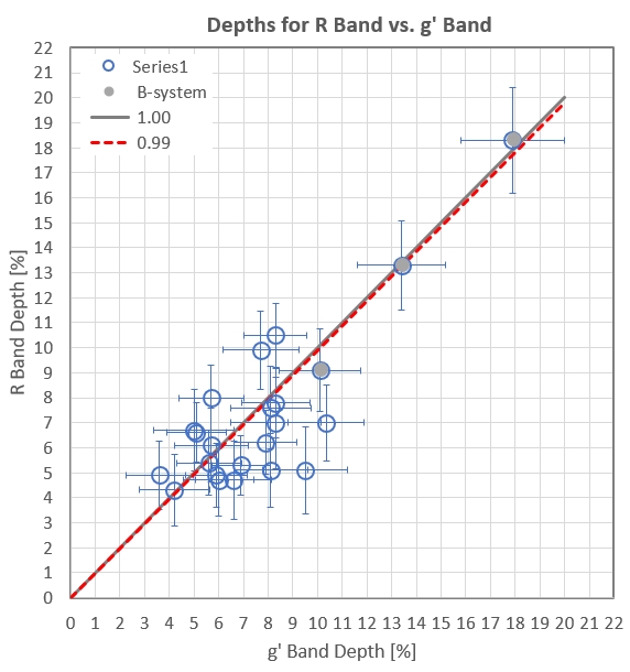
Figure 6. Scatter plot for R band vs. g' band dip depths
with a best-fit slope = 0.99 (red dashed line), based on the
assumption that the SEs for a dip measurement were the same for
both bands (different for different dips). One dip ratio was
identified as an outlier and has been rejected.
Unequal SEs for V and Y
Now let's evaluate some of the assumptions associated with adopting
measurement SEs to be the same for both g' and R bands.
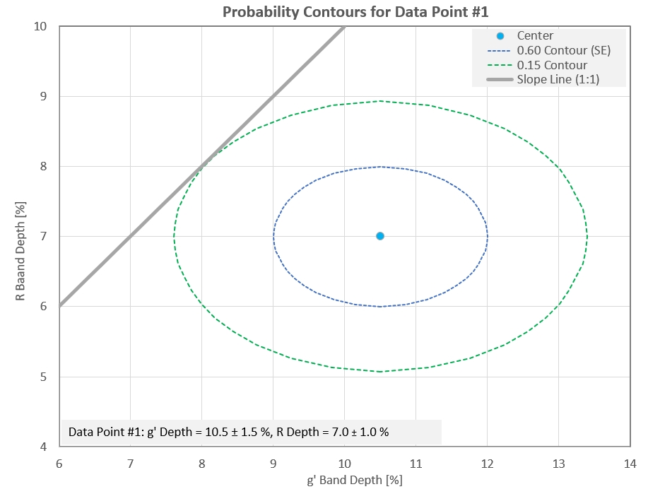
Figure 7. Actual probability function for g' and R band
measurement SEs for the first data point.
Evaluating the slope fit involves determining the highest
probability that is intercepted for each data point's probability
function. For data point #1 and a 1:1 slope the greatest probability
intercepted is 0.15. That probability isopleth is shown in the above
figure. Notice that the probability isoplet is oval, not circular.
Referring to Fig. 2, when both measurements are assigned the same SE
value (the average of both measured SEs) the highest probability
intercepted is 0.164. These two probabilities are surprisingly
similar. This suggests that choosing a circular probability
function, using an SE that is the average of the two measured SEs,
provides a suitable probability for a slope model fit, for each data
point.
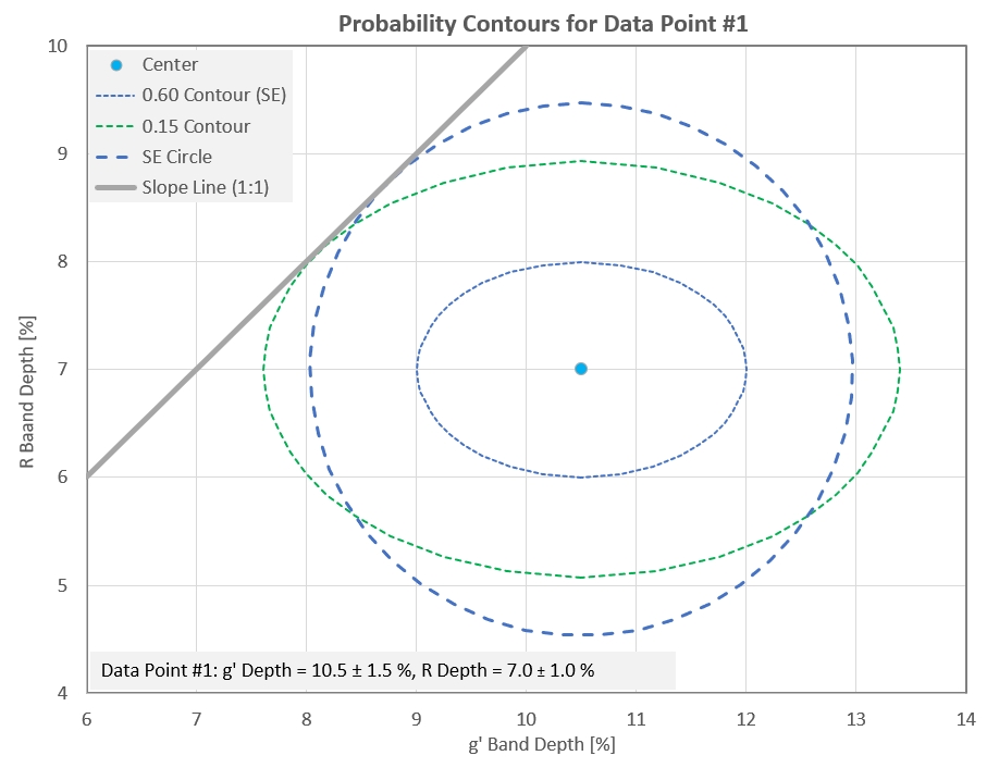
Figure 8. Same as Fig. 7 but with circle added,
corresponding to both measurements having an SE equal to the
average of their measured values.
To verify the approximate equivalence of using an average of
measured SEs as replacements for both measured values (when
performing a slope fitting procedure) it would be necessary to
perform laborious analyses, such as the one that led to Fig. 7. I
haven't decided if I want to spend my time doing this. Until that is
done by someone I will adopt the provisional position that assigning
an average SE to both X and Y measurements will lead to a correct
best-fitting slope.
Conclusion
This
References
Deming,
____________________________________________________________________
This site opened 2024.01.26. Nothing on this
web page is copyrighted.