Sample data submission showing required format.
What's New? is a web page that records changes to
the various
AXA web pages.
Note: ' symbol indicates AXA
fit value, not the "official" value
To see the light
curve plots for an exoplanet,
click on the exoplanet's
name (if it shows a link).
To
download an ephemeris spreadsheet
(Excel) that shows
transit times for all
the BTEs for an observer's site coordinates,
click here: BTE Ephem.
To
see the light curve plots
for TransitSearch candidates,
click TransitSearchLightCurves.
To see the TransitSearch
list of possible
transit times click
TransitSearch
(&
use the "Candidate Assignments"
link).
Abstract for the AXA Web Pages
This web page is a "public domain" archive for
amateur observations of known "bright transiting
exoplanets" (BTE), where "bright" means V-mag < 14.
My intent is to "preserve" amateur
observations at one convenient location and to promote
sharing
exoplanet observations by many
observers to help in the search
for anomalies that might lead
to a greater understanding of
exoplanet systems. Some light curves
(LCs) are of transits and
others are out-of-transit (OOT).
The archive manager will enhance
the LC by correcting for temporal
trends and air mass curvature
using the non-transit portion of data.
A line-segment fit will be superimposed
on the LC measurements.
Each LC will be accompanied by a listing
of mid-transit time, transit length,
transit depth and an indication
of whether the transit was early or late.
A web page is devoted to each exoplanet,
with the most recent LCs at the top.
Observers of TransitSearch candidates are
welcome to submit observations. It's OK
that most of them will be featureless; this
is useful information. A web page is devoted
to LCs for TransitSearch candidates. It
is anticipated that later in 2008 most of the data
on the AXA will be transferred to the Caltech NStED archive.
The fate of this web page will depend on how many of the
AXA features are present at the NStED/AXA.
Links
Internal to this Web Page:
Best for this Season
Purpose for this
Archive
Observation Submission
Format
Sampe of Archive
Processed
Product
Explosive Growth
of Exoplanet Discoveries
Patterns to Look For
Observing Philosophy
Aperture vs. Technique
Comment on Correcting
LCs for Slope and Curvature
Ground Rules for Professional
Use of Data Files
Contributors
Related Links
Many exoplanets are "in season" in the winter months. HD 17156 continues to intrigue astronomers, professional and amateur alike. It is well situatied for winter observing, but with a period of 21.2 days each transit becomes a high-value target. The next few opportunities are December 19.88 (Europe) and January 10.10 (Europe and USA). HAT-P-8 is the latest discovery but it is observable for only 5 hours in mid-December (setting through 20 degrees elevation before midnight). WASP-11 and the newly-announced WASP-12 are perfectly situated for December observing and they need to be observed. HAT-P-9 needs observations (none in the AXA) but it's an early morning object. XO-3 is perfectly situated for December and January observations, but it is well characterized so I'm unaware of scientific value in observing it this year. XO-2, 4 & 5 are January and February objects, the 4 & 5 need observations. HAT-P-9 is a morning object, and so far the AXA has no observations for this BTE. GJ 436 is an early morning object, and it will merit observing for years to come.
This archive was promted by the fact that amateurs have no place to submit
their
observations of exoplanet
transits where they will be
processed and displayed
in a useful format. Since it is
scientifically important to preserve
a historical record of transit light
curves (LCs), and since LCs that are
only present at an individual observer's
web page are unlikely to be preserved
for later use, there is an unmet need
for an archive that collects amateur LCs
and presents them in a uniform format. Such
an archive will grow in value and could become
a useful resource many years in the future. Only
a handfull of amateurs are associated with
a professional group of astronomers, where
archives are preserved, and their LC archive
is not in the public domain. The AXA is open
for anyone to submit observations that are likely
to be added to the AXA web pages and maintained
as a historical archive.
The structure of the present archive allows for easy browsing for the purpose of visually searching for patterns that would otherwise be difficult to detect. I anticipate that professional astronomers with their own archive (not in the public domain) will glean information from this one as they search for patterns that can only be done with large amounts of LC data. In this way amateurs with good observing skills can contribute to the professional astronomy community's growing understanding of exoplanet systems, and possibly produce interest in anomalies that could lead to the discovery of additional exoplanets in the same exo-planetary system.
This web page describes how anyone who has observed an exoplanet, and produced a light curve (LC), can submit their observations and have them added to the archive. As the archive manager I will assess the quality of the data and if it looks acceptable (99% of submissions are acceptable) I will proceed to process it. Baseline systematics will be assessed and a fit to the data using a line-segment transit model will be over-plotted on the measured data points. The resulting LC plot will list mid-transit time, transit depth and transit length. Measured mid-transit time will be compared with an ephemeris predicted time. A notation may be made on the LC plot showing 2-minute RMS of the individual measurements.
When many transits are present on a web page devoted to an exoplanet, and ordered with the most recent LC at the top, it is easy to notice the following patterns: transists occuring early or late (implying a need for refining the orbital period), depths varying in a systematic way with filter (related to star spectral type and center miss distance) and transit length varying over time. Some of these patterns can be used by anyone to search for other exoplanets using mid-transit timing anomalies, called "transit timing variations" (TTV). Other patterns may justify a reconsideration of stellar limb darkening and center miss distance. A search for another exoplanet in the same system can also be performed using the OOT data that might contain small depth features that repeat with a different period than the main transits. Many archives exist with exoplanet transit information, but none are in the public domain, and perhaps none are structured in a way that is convenient to use for the purposes just mentioned. This web page is meant for those who are not associated with professional teams that maintain a "secret" archive.
This section used to include instructions for preparing a data file for
submission to the AXA,
but it has been moved to a separate web
page: DataFormat. I'll simply
show an example of a properly formatted data
file and refer you to the above link for explanations.
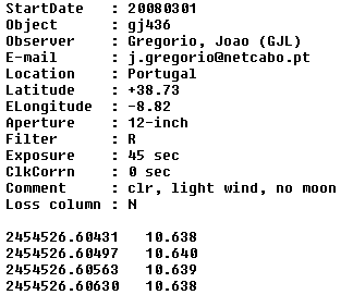
Sample
data submission showing
required format.
Here's an example of my preferred filename convention: 20080301-gj436-GJL.txt.
It
conveys the information that
the observations began
on the date 2008 March 1 (UT), the
object was GJ 436, and the
observer's 3-letter "observer code" is GJL (details
on the other web page). Attach this file to an e-mail
sent to:
a x
a @ b r u c e g a r y . n e t
[remove spaces
between characters]
Sample
of Archive Processed Product
Two light curve formats will be presented for each data submission (starting
May
1). There will be a top panel LC,
a bottom panel LC, and a 4-row information
section between the panels.
In the following example
the top panel is a version of the
data with the two principal systematic
errors removed (temporal
trend and air mass curvature). This is
the format used by professional astronomers.
Since amateurs have larger systematic
errors I have included the lower panel
to show the same data before removal of
these systematic errors. The lower
panel also shows a air mass and "loss" plots
(described below). For this example we
can readily see that the early data were made at
very high air mass, which explains the greater noisiness
of the data and extreme air mass curvature.
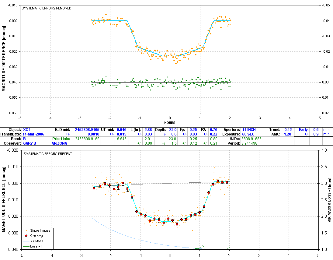
The middle section states that the transiting object is XO-1, using a
R-band filter, and mid-transit occurred on March 14, 2006 UT. The 7-segment
model fit (explained in detail at model) has a mid-transit
HJD of 2453808.9165
± 0.0010. This
corresponds to UT = 9.946 ±
0.015 (based on the date and source
coordinates). The ephemeris
predicted HJD and UT are also
shown in the 3rd row (green). The
transit length was measured to be
L = 2.88 ± 0.03 hours, which is slightly
longer than the consensus value of
2.91 hours. The transit depth is 23.0
± 0.6 mmag, which is the same as the
consensus value. Fp is the fraction of
time the transit is "partial," defined using
contact times as Fp = ((t2 - t1) + (t4 - t3))
/ (t4 - t1). The solution for Fp is 0.25 ±
0.03. F2 is the ratio of depth at t2 and t3 divided
by the depth at mid-transit, and for this solution
F2 = 0.76 ± 0.22. The ephemeris HJDo and Period
(used to calculate expected mid-transit time)
are shown. The fitted temporal trend (-0.42 mmag/hour)
and air mass curvature coefficient (+1.20 mmag
/ airmass) are given. The entry "Early: 0.6 ± 0.9 min"
states that mid-transit was earlier than the
ephemeris time by 0.6 minutes. You'll note that
blue entries
are specific to the submitted observations
and green
entries are from an ephemeris or
a consensus of previous observations. The
upper panel includes a plot of departures
of the measured magnitudes from the model
fit, or "O-C" (observed minus computed). The
lower panel's large red circle
data, with SE bars, are averages of non-overlapping
groups of either 5, 7, 9, 11, 13 or 17 individual
image values. At the bottom of the lower panel
is a green trace showing "losses" offset so that
their magnitude value is 1.0 when losses are zero
(as read on the right side). Losses refer to the effect
of clouds, dew on the corrector plate, wind shaking
the telescope enough to broaden the point-spread-functionof
all stars so that some of the photo electrons
spill out of the aperture circle. For this
example there was dew formation on the corrector
plate that was evaporated with a hair dryer
at 1.1 UT, and another dew formation just prior to
the end of observations (~0.1 magnitude loss in both
cases).
I've adopted this presentation because it is quicker to produce than previous
versions. If
Caltech really does assume responsibility
for the AXA it won't
be open for public submissions for
at least 6 months, and during that
time I want to minimize my workload.
A program is used to perform chi-square
fitting of submitted data and
records a file that is easily imported to the
spreadsheet which is screen captured as
an image file for import to a web page. The entire
process is much faster than the hand solution
searches I used to perform, and this
will enable me to accept more data submissions.
If you preferred the other versions,
requiring hand-entered values for such things
as mid-transit time, length and depth,
then I hereby apologize for abandoning
them.
As stated above,
a description is given of
the very simple transit "model"
used for fitting the submitted
measurements at model
fitting.
Explosive Growth of Exoplanet Discoveries
The number of bright transiting exoplanets has doubled in the past year (mid-2006 to mid-2007). There may be an equal number of undiscovered transiting exoplanets among the list of 246 exoplanets discovered spectroscopically (i.e., from radial velocity variations) found on the TransitSearch.org web site. There are plenty of observing opportunities for amateurs not associated with a wide field camera survey team, like the XO Project. Even an "arm chair" amateur astronomer can become engaged with a study of existing observations. There is merit in collecting all LC observations for each object and searching for patterns. One pattern would be transit timing variations (TTV) of mid-transit times; another would be a search for shallow transits during OOT times; and a search could even be made for LC structure within a transit or just outside transit by combining and averaging many LCs. For example, an exoplanet with rings may produce a brightening just before ingress and just after egress. Some day there may be a central archive where ALL exoplanet LC observations can be found. It is appropriate for either NASA or NSF to maintain such an archive. Caltech's IPAC archive would be an appropriate place for this addition. It would also be appropriate for a European institute to host the archive. Until this happens I would like to urge my fellow amateur astronomers to share their LCs on this public archive.
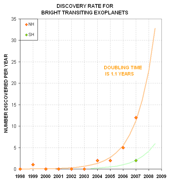
The rate of discovery of "bright transiting exoplanets" is growing exponentially with a doubling time of 1.1 years. The discovery rate of BTEs in the northern celestial hemisphere (orange) can serve as an estimate for what can be expected for the discovery rate of BTEs in the southern skies. By the end of 2008 there may be ~52 known BTEs using this model.
The first 21 BTE discoveries were in the north celestial hemisphere because until recently the wide field search cameras were only in the northern hemisphere. Now that southern hemisphere cameras are in operation it won't be long before there will be about as many BTEs in the southern skies. If we assume the discovery rate curve for BTEs in each celestial hemisphere has the same shape (doubling time) then the discovery rate curve for the NH (orange trace in above figure) can be shifted 2.4 years to show what can be expected for SH discoveries versus time (green trace, in above figure). By the time the list of northern sky BTEs is complete to 14th magnitude the discovery rate curve will flatten out to some unknown limit which will depend on how many long period exoplanets are there to be discovered. This is unlikely to happen before the end of 2008, when this model predicts that we will know about 52 BTEs.
If an exoplanet has a debris system in the same orbit (e.g.,
volcanic ejecta surrounding
and perhaps following the "hot Jupiter"
planet) the debris particles
will
"forward scatter " and produce brightness
enhancements before ingress and after egress.
The pre-ingress and post-egress brightenings should
have a different brightening amount and shape.
This effect is likely to be too small for detection
using amateur observations but unusually large, transient
ejection events should not be ruled out.
If an exoplanet has a ring system the ring particles will also "forward scatter" and produce a brightening before ingress and after egress that can last several minutes. In 2004 Joe Garlitz and I independently noticed that amateur LC observations of TrES-1 showed a small brightening (~5 mmag) after egress, lasting ~10 minutes. Ron Bissinger did an exhaustive statistical analysis of many TrES-1 LCs and concluded that the feature was statistically significant. Subsequent HST observations failed to confrim the feature so we are left to assume that the apparent brightenings were a statistical fluke. All exoplanets should be inspected for such a feature even though the effect is probably going to be much smaller than amateur observations could detect (< 0.3 mmag according to Brown and Fortney, 2004 and Otha et al, 2008).
An exoplanet may have a moon of its own, and if its large enough it could produce a small fade either before ingress or after egress. This would probably be noticed as a change in mid-transit time since on any one transit the moon will affect only an ingress or only an egress for a given transit. Brown et al (2001) searched for this effect with HST observations of HD 209458 and found nothing. Again, amateur observations are likely to be insufficiently precise to observe such an effect unless the moon is comparble in size to the hot Jupiter.
Mid-transit time can vary if the exoplanet is accompanied by another exoplanet in an orbit with a period resonance, such as 2:1, 3:2, etc. For exoplanets with a long record of transit timing measurements these timing anomalies should be searched for.
Transit length and depth can vary if the transiting planet is close to "grazing" and another planet in a nearby orbit that inclined differently causes changes in the transiting planet's inclination. This was thought to be the situation for GJ 436 in January 2008 (Ribas et al, 2008a; Ribas has since withdrawn this suggestion in the light of later observations that offered a simpler interpretation). Still, any exoplanet with an "impact parameter" close to 1, such as GJ 436, TrES-2, TrES-3 and HD 17156, should be viewed as candidates for transit property changes due to inclination changes caused by another exoplanet in a resonant orbit.
If an exoplanet has Trojan planets (same orbital period but located at longitudes 60 ahead or behind) there may be a detectable fade at times that are offset 1/6 of a period before or after the main exoplanet transit event. For hot Jupiter periods of 3 days, for example, the Trojan features will occur ~12 hours before or after the ephemeris transit. This offset is longer than any single transit observing session, so only the OOT observations can be used for this purpose.
Sunspots will produce a small brightening during the interval Contact 2 to Contact 3 but they'd have to be large to be detected by amateur hardware. If a feature is seen on one LC it may not be seen on others unless the periods are the same (period of exoplanet orbit and period of rotation at the sunspot's latitude).
On a typical night at least one of the BTEs will undergo a transit. On those nights when none are observable check the TransitSearch candidate list. If no known BTE transits are on the schedule, and the TransitSearch candidate list is unappealing for the night, there is merit in conducting OOT observations of a BTE. Preference can be given to exoplanets that are ~1/6 of a period away from transit, since that's when Trojans would produce their transit signatures. Another consideration is "impact parameter" - the ratio of closest approach miss distance to star radius. Small impact parameters are good candidates for second exoplanet transits in outer orbits. Small impact parameter systems have flatter bottomed transit shapes (i.e., contact 1 to contact 2 is short compared with contact 2 to contact 3).
If your interest is in a search for LC transit shape anomalies, either brightenings or fadings before ingress and after egress, then give preference to observing a bright exoplanet. Although scintillation will be the same regardless of a star's brightness, the SNR (caused by Poisson noise) will be better for brighter stars.
May I suggest that you "adopt" an exoplanet that transists near midnight
and
simply observe it every clear
night. After inspecting it
for anomalies that you can hope
are real and repeating with an
unknown period, the overall
OOT shapes can at least be used to
learn about your observation's
systematics. For example, an
OOT set of measurements would produce
a LC that is "flat" and "horizontal"
if no systematics were present.
However, if your polar axis is slightly
mis-aligned (>0.1 degree),
and if your master flat field is imperfect,
the LC will have a sloping trend of as
much as several mmag per hour. If a small
scale feature in the master flat is imperfectly
represented (such as a dust
donut) then features could be superimposed
on the sloping trend line. A hot or
cold pixel (or imperfect master dark frame)
could produce the same features. Another
systematic, that is quite common, is for
the OOT LC to be curved in a way that is related
to air mass. This arises when the exoplanet
star is not the same color as the reference
star (or the average color of the reference stars,
if ensemble photometry is employed). If your
OOT observations produce an LC with a curvature
that is correlated with air mass then you may want
to give attention to reference star color when
choosing reference stars.
I have slowly come to appreciate some fundamental differences between
the kind of variable star observing and image analysis performed for the
AAVSO versus that required for exoplanets. Occasionally a new observer will
be handicapped by adhering to traditional variable star observing procedures.
For these observers I recommend reading
a web page I created that describes
the observing task differences, and
how observing strategy and image analysis
should be adjusted on behalf of the exoplanet
task: Exoplanet Stars
Are Not Variable Stars.
Whenever someone asks "what hardware is needed for observing exoplanet
transits" I try to explain that a more relevant question
to ask is "how competent an observer must I be for observing
exoplanet transits?" This idea has been dramatically demonstrated
by an observation
that has recently come to my attention. Petr Svoboda
(Czech Republic) used a 1.33-inch aperture "telescope"
(actually, a 34 mm aperture camera lens) with a SBIG ST-7
CCD camera to obtain the following light curve:
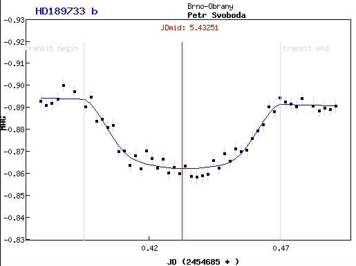
Small aperture light curve
made with a 1.33-inch "telescope" (34 mm camera lens).
Another impressive demonstration comes from Gregor Srdoc (Croatia) who
used a 2.5-inch camera lens attached to a regular DSLR
camera (12-bit) to measure a 9.5 mmag depth transit of
XO-4. The message from these two examples is that "aperture
isn't everything" because technique is important regardless
of aperture. Technique is based on an understanding of observing
concepts, image analysis and data analysis. I believe that it's
difficult to teach any of this because the best way to learn is
to "flounder" with whatever hardware is available! So my advice to
anyone who wonders what hardware is needed for exoplanet transit observing
is to change the question to "how willing am I to learn from floundering
with whatever hardware I have?" And remember, floundering is fun!
Comment on Correcting LCs for Slope and Curvature
I disagree with the custom of professional astronomers who present transit light curve plots that have been "corrected" for a temporal trend and an air mass (extinction) correlation. The viewer has no clue about the magnitude of either correction when viewing a plot with those effects removed. As I show in my book Exoplanet Observing for Amateurs (Chapter 14, pg 82) the presence of these corrections influence such "transit parameters" as depth, shape, length and mid-transit time. There usually is a locus of points in slope/curvature parameter space (temporal slope and air mass coefficient) having equally good fits yet yielding varying results for transit parameters. Because of my experience with hand-fitting the LCs by experimenting with values for slope and curvature, and seeing the effect these choices have on transit parameters, I am reluctant to accept elaborate solutions for planet radius in a paper where there is no discussion of the slope/curvature fitting ambiguities. It's potentially misleading to simply experiment with the slope and curvature coefficients until the LC looks good, and then proceed with an elaborate chi-squared analysis seeking solutions for planet size, inclination, limb darkening, etc. without also including the slope and curvature coefficients as independent variables. Consider the following innocent-sounding description: "We then fit a linear function of time to the pre-ingress and post-egress data. A function of time proved to be a slightly better fit than the more traditional function of airmass." (reference available upon request).
I have adopted the practice of preserving the uncorrected photometry data points while applying the temporal trend and air mass correlated solutions to the "model fit" trace. These LCs may not look as pretty as the ones professionals publish, but they convey more information and are a more honest representation of the LC that was measured. Therefore, if you're used to seeing the pretty LCs with slope and curvature corrections removed, think twice before passing judgement on the sloped and curved LCs you see on the AXA web pages for each exoplanet.
I plan on adding a link to an illustration of quantitative effects upon
transit
parameters when the slope
and curvature corrections are
treated carelessly.
Ground Rules for Professional Use of
Data Files
The description of various versions of these "ground rules" can be found at: GoundRules A short version that will be included in the header of those data files that are transferred to Caltech's IPAC computer (NStED archive), in late 2008, is presented here:
"Downloading of amateur data files is unrestricted. However, since these data are unpublished it is recommended the observer be contacted prior to use of data. The observer may be aware of specific aspects of the data that should be taken into consideration when interpreted, such as seeing, clouds, wind, scintillation, clock-setting procedures, optimized photometry apertures, etc. If these data are to be used in a publication, it is requested that the observer be acknowledged by name along with a brief description of the hardware used."
AXA and TransitSearch contributors (top of list is the most frequent contributor). The contributor list is divided into two categories: "active and "inactive." To be "active" an observer must have contributed at least one observation during the previous 6 months (the date of the observation is not relevant). (Three of the observers on the lists are more active than they appear since they are contributors to the XO Project and only some of their observations can be submitted to the AXA; they are Foote, Gregorio and Vanmunster.)
Total number of LC submissions ...... 405
Active Observers & their Code Obs'g Site TotNr Submissions (during previous 6 months)*
Manuel Mendez
(MQZ)
Spain
27 8b25,8b16,8b14,8b11,8b06,8b01,8829,8825,8826,8814,8812,8812,8731,8729,8724,8710,8710,8709,8708+
James Roe
(ROE)
Missouri
26 8918,8918,8903,8819,8801,8808,8804,8729,8729,8729,8615,8617,8612,8611,8528,8525,8522,8521,8521+
Cindy Foote
(FC2)
Utah (USA)
54 8c11,8b18,8b17,8a29,8903,8903,8624,7b13,8607,8607,8607,7a25,7a25,7a09,7a09,7215
&
many others
Veli-Pekka
Hentunen
(HVP) Finland
21
8a29,8b06,8b06,8b06,8b06,8b01,8b01,8b01,8a29,8a29,8a29,8a18,8a18,8a18,8a18,8a18,8a18,8a18,8a17+
Anthony Ayiomamitis
(AA2) Greece
15 8b26,8b22,8a08,8a05,8906,8903,8902,8709,8628,8626,8613,8606,8603,8528,8503
Bruce
Gary
(GBL)
Arizona,
USA 72
8c10,8b30,8b14,8b08,8b02,8a28,8a22,8a18,8a17,8a15,8a14,8701,8602,8603,8528
Ramon Naves
(NR2)
Spain
34 8b29,8a06,8915,8909,8818,8818,8814,8814,8803,8803,8719,8622,6507
Gregor Srdoc
(SG2)
Croatia
17 8a27,8630,8625,8609,8601,8602,8528,8514,8512,8507,8503
Joao Gregorio
(GJ2)
Portugal
22 8c20,8c16,8c14,8c05,8a05,8127,8120,8302
Yenal Ogmen
(OYE)
Cyprus
7 8a11,8907,8922,8724,8710,8702,8630
Standa Poddany
(PS2)
Czech Republic
6 8a23,8905,8905,8827,8716,8627
Fabio Salvaggio+
(SFV) Italy
5 8901,8901,8706,8616,8614
Enric Forne
(FE2) Spain
4 8c16,8929,8929,8929
Ricard
Casas
(CRI) Spain
4
8929,8929,8929,8929
Nicolaj Haarup
(HNI)
Denmark
5 8413,8320,8319,8318
Toni Scarmato
(SFI) Italy
3 8c06,8b20,8814
Miguel
Rodriguez
(RMU)
Spain
3 8809,8512,8415
Peter Kalajian
(KP2) Maine
2
8908,8911
Gustav Muler
(MG2) Canary Islands
2 8914,8301
Tonny Vanmunster
(VMT)
Belgium
34 8511,8511
Darrel Moon
(MD2) Utah
3 8704,8703
Giuseppe Marino
(MG3)
Italy
2 8717,8616
Josep M Coloma
(CJI) Spain
1 8c16
Petr Svoboda
(SP2) Czech
Republic 1 8b03
Ramon Costa
(CR2) Spain
1 8929
Joal Bel
(BJ2) Spain
1 8929
Xavier Puig
(PX2) Spain
1 8929
Fernando
Tifner (TF2)
Argentina
1 8924
Stelios
Kleidis
(KSM)
Greece
1
8607
Bart Staels
(SBL) Belgium
5
8207
Colin Littlefield
(LC2)
Indiana, USA 1
8B22
* Date code is YMDD. Example #1: 20080317 = 8317; Example #2: 2007 December 31 = 7c31 (think HEX). Starting July 8 entries will be for date of submission, not observing date.
Some of the 3-letter observer codes for the active observers have links to description of hardware (and picture of hardware with observer).
Note: I salute the Europeans for their involvement with exoplanet observations and contributions to the AXA. Most of the active contributors are Europeans, although the most prolific contributor is in Utah.
RelatedLinks
Exoplanet
Observing for Amateurs
(book)
Useful
spreadsheets (BTE_ephem.xls, etc)
Jean Schneider's Extrasolar Planet
Encyclopaedia
Greg Laughlin's TransitSearch
archive
NStED (Caltech's
NASA/IPAC/MSC
Star and Exoplanet
Database)
Bruce's
AstroPhotos
Resume
WebMaster: B.
Gary.
Nothing
on this web page is
copyrighted. This site
opened: 2007 August 06, Last Update: 2008.12.20