ALL-SKY PHOTOMETRY FOR AMATEURS
USING SDSS FILTERS g'r'i'
FOR DERIVING BVRcIc MAGNITUDES
Bruce L. Gary; Hereford, AZ, USA
2009.10.03
This web page is meant for amateurs wanting to perform all-sky observations
of uncalibrated star fields for the purpose of deriving standard magnitudes
(BVRcIc) from observations made with the SDSS filter set (g'r'i'). I must
warn that this task is not easy, and I don't recommend it to anyone who
has not already performed all-sky observations using the BVRcIc filter set.
Links internal to this web page
Preface
Basic photometry equation
Getting star fluxes
Spreadsheet analysis
Unknown star
field plots
Unknown target
star magnitudes
Reality checks
Related links
PREFACE
"A Landolt star with V-mag = 8.61 is measured
to have a flux of 264765 counts near transit. An unknown target star at the
same elevation is measured to have a flux of 38767 counts. The brightness
ratio is 6.83, which corresponds to a magnitude difference of 2.09. The
unknown star is fainter, so it must have V-mag = 10.70. What's so difficult
about all-sky photometry?"
|
I like introducing the concept of all-sky photometry with
the above example. It captures the notion that the concepts involved are
simple, and easily understood. However, it is misleading because to do all-sky
photometry right there are many details that have to be managed carefully
and systematically. I have created several tutorial web pages for amateurs
wanting to perform all-sky photometry. I do this, ironically, knowing that
probably no amateur will ever be successful with this daunting endeavor.
My persistence in this was originally prompted by an encounter with the notorious
"CCD Transformation Equations" (CCD TEs) promoted by the AAVSO for use with
differential photometry of a variable star with nearby calibrated stars.
I use the word "encounter" in the previous sentence because I knew that
the CCD TEs were an ungainly and error-prone procedure for doing something
basically simple. After I derived the CCD TEs from basic concepts, to prove
that I understood them, I formulated a simpler procedure that was more intuitive,
less prone to errors and capable of showing when problem stars were present.
I argued that the old CCD TEs may have been a good idea when log tables and
slide rules were in use, but with PCs and spreadsheets on every amateur's
desk the time was right for a modernization of differential photometry that
employ corrections for a telescope system's star color systematics. Most
of my early tutorial web pages addressed this need, but lately I have become
fascinated with extending these concepts from differential photometry to
all-sky photometry.
Performing all-sky measurements using BVRcIc filters to derive BVRcIc magnitudes
is difficult, so imagine the extra complication of using g'r'i' filters
for deriving BVRcIc magnitudes! The CCD TEs are not designed for this, but
my procedures are easily adapted for the task. That's what this web page
is all about.
Amateurs are probably going to migrate to the use of the SDSS filter set
as they realize their advantages, following the lead of professionals already
making the switch. However, the need for magnitudes in the traditional bands
will remain. One path to the desired magnitudes is to first calculate g'r'i'
magnitudes, then convert them to BVRcIc magnitudes using equations derived
by professionals. I suggest using this as a check of a more direct procedure:
calculating BVRcIc directly from g'r'i' flux measurements.
The following two plots show transmission functions for the two filter
sets, BVRcIc and g'r'i'z'.
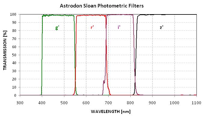
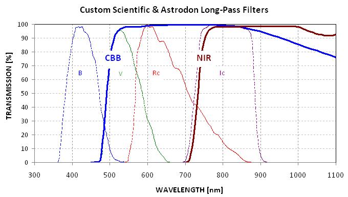
Figure 01. Filter transmission functions. CBB and NIR filters
are not relevant to this web page.
1. BASIC PHOTOMETRY EQUATION
Everything I do with photometry is based on what I call the "basic photometry
equation" for relating measured star flux to magnitude:
Mag = Z - 2.5 × LOG10
( Flux / g ) - K' × AirMass + S × StarColor
(1)
where Z is a zero-shift constant, specific
to each telescope system and filter (which should remain the same for
many months),
Flux is the star's flux (sum of counts associated
with the star). It's called "Intensity" in MaxIm DL,
g is exposure time ("g" is an engineering term
meaning "gate time"),
K' is zenith extinction (units of magnitude),
S is "star color sensitivity." S is specific
to each telescope system (and should remain the same for amny months),
StarColor can be defined using any two filter bands.
B-V is in common use; I will use a version based on g'-r' on this web page.
This general equation is true for all filter bands (even unfiltered),
though there are different values for the constants for each filter.
For example,
V = Zv - 2.5 × LOG
( Flux / g ) - Kv' × AirMass + Sv ×
StarColor
(2)
R = Zr - 2.5 ×
LOG ( Flux / g ) - Kr' × AirMass + Sr ×
StarColor
(3)
Similar equations exist for bands B and I.
Notice that in a "basic photometry equation" for a specific
filter there are two terms associated with a telescope system that should
remain constant (until hardware configuration changes are made). This is
illustrated for V-band:
V = Zv - 2.5 ×
LOG ( Flux / g ) - Kv' × AirMass + Sv × StarColor
(4)
Zv and Sv are highlighted in green, and the task of "photometrically calibrating
a telescope system" amounts to evaluating these two constants for each filter
band of interest.
Notice that nothing in the above equations specify which filter is to be
used for measuring "Flux". For example, star flux can be measured using
a g' filter, in which case the two constants Zv and Sv are to be associated
with g' fluxes. Also notice that StarColor can be defined using any two
filters, so g'-r' would be a logical StarColor definition when the g'r'i'
filter set is used. As will be described below the parameter Sv can be derived
by plotting something versus StarColor and solving for the slope, which
can be equated to Sv. Independently, Zv can be determined by noting the
average offset error for a trial Zv value and adding it to that trial Zv.
Here's an example of what is sought:
V(g') = 19.61 - 2.5 ×
LOG ( Flux(g') / g ) - Kv' × AirMass - 0.784 × StarColor
(5)
where StarColor = 0.61 ×
(g'-r') - 0.294 when g' and r' are available, or
StarColor = 0.57 × (B-V) -0.33 when g' and r' are
not available.
The way to "read" the above equation is that a V-band magnitude can be derived
from g' observations of star flux, Flux(g'), when StarColor is defined by
either of the above two definitions. Note that the two definitions of StarColor
are designed so that it is zero for a typical star (the median star in the
Landolt list of 1264 well-calibrated stars). This allows the star color term
to be neglected when no color information is available, or when deriving it
will not be possible. For all-sky photometry calculations in which accuracy
is important the StarColor term cannot be neglected, and most of the procedures
described on this web page deal with this matter. The observer has to determine
Kv' (atmospheric extinction at zenith) for the night in question if the target
star and the calibrated star fields are at different air masses (if they're
at the same air mass then this term can be dropped). If only small air mass
differences are involved then the atmospheric extinction coefficient can
be assumed (based on what's typical for the observing site). For example,
at my site Kv' = 0.21 [magnitude/airmass] for g'-band measurements.
For quick-and-dirty hand calculator determinations of approximate magnitude,
which I often do while observing, it is convenient to 1) neglect the star
color term, and 2) use a site-typical zenith extinction value for the filter
in question. These two simplifications yield a set of very simple equations
for converting star flux to magnitude, as illustrated by the following set
that applies to my observing site and hardware:
B(g') = 20.30 - 2.5 × LOG ( Flux(g')
/ g ) - 0.21 × AirMass
V(g') = 19.61 - 2.5 × LOG ( Flux(g')
/ g ) - 0.21 × AirMass
Rc(r') = 19.81 - 2.5 × LOG ( Flux(r') / g
) - 0.15 × AirMass
Ic(i') = 18.61 - 2.5 × LOG ( Flux(i') / g
) - 0.09 × AirMass
Use of these very simple equations are typically accurate to the 0.1 magnitude
level for Rc and Ic, and slightly worse for B and V.
2. GETTING STAR FLUXES
When using the BVRcIc filter set it is adequate to use only the Landolt
star fields for calibrating a telescope system. But when SDSS filters are
used it is necessary to observe both the Landolt star fields and stars that
have been calibrated using SDSS bands (u'g'r'i'z'). This latter need is met
by the Smith et al, 2002 publication ("THE u'g'r'i'z' STANDARD STAR SYSTEM"
AJ, 123, 2121-2144, 2002 April). This publication lists 158
stars with SDSS magnitudes measured at the USNO Flagstaff, AZ observatory.
It also presents conversion equations for going between u'g'r'i'z' and BVRcIc.
I have created ASCII files for both the 1284 Landolt stars and 158 Flagstaff
SDSS stars in a format that can be imported to TheSky/Six, which allows
for display on star fields of any of the magnitudes of these two databases.
This TheSky/Six capability is important for both the planning of precise
positioning of star fields during the observing phase and the notation of
magnitudes on printed star fields during the analysis phase.
Care must be made in planning an observing session for the purpose of calibrating
a "telescope system" (defined as the telescope, focal reducer lens, filters,
and CCD at a specific observing site - all of which have unique spectral
transmission and response functions). A range of air mass (AirMass) conditions
is needed for deriving accurate Z values. Calibration star fields must include
both Landolt stars and Flagstaff SDSS stars (a few stars have all bands calibrated).
My preferred exposure sequence consists of a set of 8 images taken with
a g' filter and another 8 exposures with r' (plus a few with CBB (clear
with blue-blocking) and NIR (near infra-red, long-pass starting at 720 nm).
Typically I will observe each of maybe 6 to 10 calibrated star fields using
the previous sequence two times (in quick succession). It's important to
position the main CCD chip's FOV for maximum number of calibrated stars,
and this usually means that there are no stars in the autoguider's FOV that
are bright enough for use. Therefore, exposure times are kept short enough
to prevent unguided telescope motion from smearing star PSF (point-spread-function).
I use 10 second exposures. Throughout the observing session any desired target
stars can be observed at times dictated by the desire for similar air masses.
Amateurs have the handicap that most calibrated stars are "faint" when
using small apertures. My aperture is 11 inches, and 10-second exposures
barely register standard stars fainter than V-mag ~12. Most stars are brighter
than this, but it is important to make use of as many calibration stars
as possible. I therefore want to employ as small a photometry signal aperture
as possible to maximize SNR. There's a tradeoff between the photometry aperture
that produces the best SNR (i.e., radius = 1.4 × FWHM)
and very large apertures which minimize most systematic errors. There's a
way to have the benefits of a small aperture's large SNR without its systematic
error penalties, but it involves a little more manual effort. A bright star's
flux is manually measured using large and small apertures and the magnitude
difference is noted in a reduction log. The small aperture is typically 2.5
× FWHM (which affords good SNR, but not as good as the 1.4 ×
FWHM SNR), and the large aperture is typically 5 to 10 ×
FWHM. The large aperture captures ~99.9% of total flux, and the small aperture
captures ~ 90%. For each image the difference in flux capture fraction can
be established accurately if a bright star is used. It is assumed that all
other stars exhibit the same flux capture fractions. Since star fluxes (and
magnitudes) can be measured with much better accuracy using the small aperture
compared with the large one an automated photometry tool should be specified
to use the small aperture for measuring all stars of interest in each of
the 8 images associated with a filter. When a CSV-file with these fluxes
(or magnitudes) are later imported to a spreadsheet the user must enter the
manually-read magnitude differences from the bright star in each image, and
the average of these differences is applied to the automatically measured
fluxes (magnitudes) for all stars. Thus, the fainter stars are measured with
the SNR of a small photometry aperture but after the "small/large aperture
correction" they have fluxes (magnitudes) corresponding to capturing ~100%
of their flux.
Note that I've equivocated by using the terms "fluxes (magnitudes)". This
is because I use the image processig program MaxIm DL, which records only
magnitudes in the photometry tool's CSV-file. I am able to convert these
magnitudes to fluxes by first adding an artificial star to each image (in
the upper-left corner), which is specified as the only "reference" star for
the photometry tool. The other stars in the FOV, such as the Landolt and
Flagstaff SDSS stars, are designated "check stars" so that their magnitues
are also recorded in the CSV-file. In this way MaxIM DL can be "tricked"
into recording the equivalent of star fluxes (since the flux of the artificial
star, used as reference, is the same fixed value in all images).
3. SPREADSHEET ANALYSIS
You have to enjoy spreadsheets to endure what follows. I don't recommend
creating one from scratch for the purposes of processing flux readings of
all-sky images. I'll make mine available and you can modify it, or get ideas
from it, if you're going to be doing all-sky analyses. The next figure is
the first page (also called "worksheet"), where CSV-files are imported.
It can handle as many as 24 stars and 18 images for a set of measurements
taken with one filter during a brief time interval.
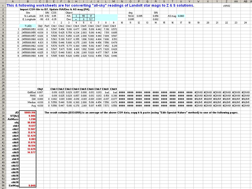
Figure 02. First page of spreadsheet where CSV-file is
imported (to cell B7). The upper section uses columns for JD and magnitudes
(relative to an artificial star) for the target ("Obj1"), the artificial
star ("Ref1") and several Landolt or Flagstaff SDSS stars ("chk1" etc).
The lower section displays results of calculations of average star magnitudes
adjusted for the artificial star's magnitude (cell U4). The values for the
rectangle of red numbers is copied to other pages.
The data illustrated in this figure are for a group of 8 g' images (plus
an average of the 8) for 9 stars at a Landolt star field centered on RA
= 03:55:17, DE = +00:05.7; four of these stars are also included in the
Flagstaff SDSS list so they have calibrated magnitudes for g'r'i' as well
as BVRcIc.
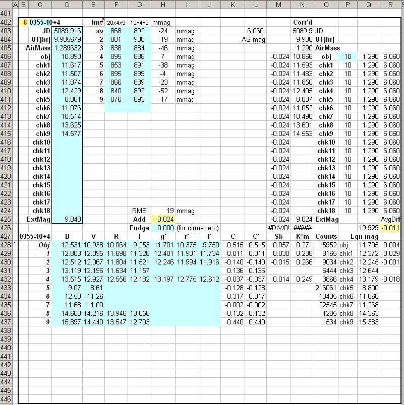
Figure 3. Second page, devoted to g' measurements used to solve
for Z and S for deriving g' magnitudes. The "red box" section of the 1st
web page is copied (values mode) to D403:D425. The large and small aperture
manual readings of a bright star in this 8-image set are entered in cells
F403:G411. The average small aperture correction is -0.024 mag (cell H425).
Magnitudes from the Landolt and Flagstaff SDSS catalogs are entered in cells
D428:J437. Star color, C, and a linearized version, C', are calculated from
g'-r' if these magnitudes exist, or B-V (i.e., Landolt). "Star fluxe per
second" is calculated for each star from its magnitude and the artificial
star's fixed flux (cells O428:O437). g' magnitudes are finally calculated
using the "basic photometry equation" and provisional values for Z, S and
K' (at top of this page, shown in the next figure). Columns labeled Sg' and
K*m are discussed in the text.
The above figure shows a small section of the second page which is devoted
to all g' measurements of many star fields. This is the 8th such star field.
The next figure shows the top of the same page.

Figure 04. Top of the page devoted to processing g' measurements
to g' magnitudes. The artificial star's flux is always 1334130 counts (cell
D5). A provisional value for Zg' is 19.918 (cell U2). A provisional zenith
extinction value for g' is Kg' = 0.207 [mags/airmass] (cell 3). A provisional
star color sensitivity coefficient for g' is Sg' = +0.118 [mags/mag] shown
in cell U5. Other descriptions are in the text.
The "ZeroShift" cell (U2) can be changed by the user (based on a "suggestion"
in cell U1). The star color sensitivity and zenith extinction values can
be changed using slide bars. A temporal trend for zenith extinction is available
for nights when the atmosphere is changing. These provisional values are
used in the basic magnitude equation for calculating provisional g' magnitudes
(in Fig. 2). Solving for Sg' (cell U5) is helped by a plot shown in the
next figure.
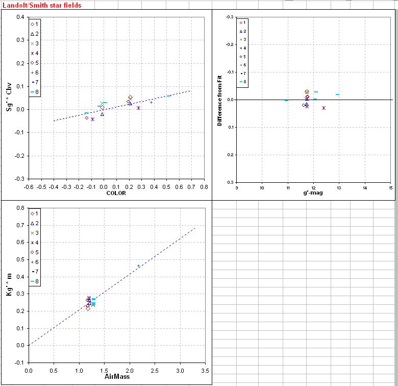
Figure 05. The upper-left plot is for a parameter whoose slope
versus star color is Sg'. A slide bar moves the slope, hinged at the median
star color, which allows for quick "eyeball" fitting. When the extinction
and zero shift parameters have good values the lower-left panel shows a
good fit. The upper-right panel shows residuals versus g'-mag.
This page can't be finalized until the next two pages are complete (g'
to B and g' to V). There are too few stars with g' magnitudes for a good
extinction solution, but there are many more stars with B and V magnitudes
that provide the main constraint on Kg'. (This will be clear, shortly.)
Solving for the best Zg' (zero shift) must await completion of the next
two pages since only when Kg' is established can Zg' be solved for.
The next figure shows the relation between measured g' magnitudes and catalog
B magnitudes, and the following figure shows measured g' versus catalog
V magnitudes.
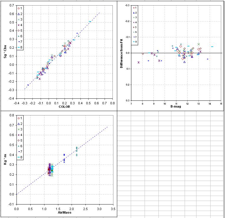
Figure 06. Counterpart to Fig. 4 except for g' measurements related
to calibration star B magnitudes. The slope for the extinction plot (lower-left
plot) corresponds to atmospheric extinction at g'-band.
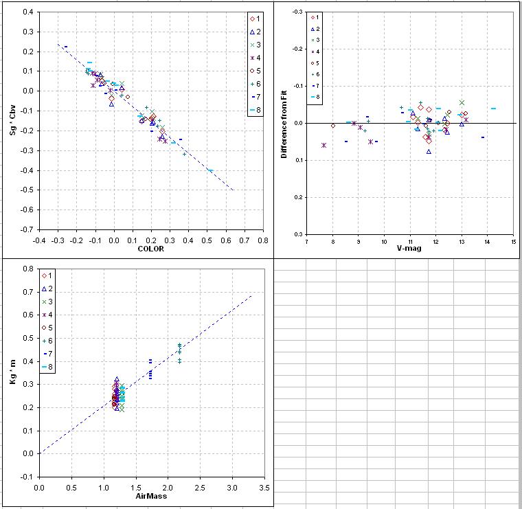
Figure 07. Counterpart to above figure except for g' measurements
related to calibration star V magnitudes. The slope for the extinction plot
(lower-left plot) corresponds to atmospheric extinction at g'-band.
Note that the extinction slopes for all three ways to use g' measurements
have the approximately the same extinction slope. The extinction slopes
for g' versus B and V should be the same as g' versus g' since the same
measured values are entered in each spreadsheet page. A weighted average
of all three estimates for zenith extinction should be used for all three
pages. For this case I adopted 0.207 [mag/airmass] for the three g' pages,
and the plots above use this value. For my observing site this is intermediate
between historical measurements of B and V extinctions (0.24 and 0.16 mag's
per airmass). This agrees with expectations since the g' filter's
passband is intermendiate between the B and V passbands.
Consider the three color sensitivity plots, reproduced here.
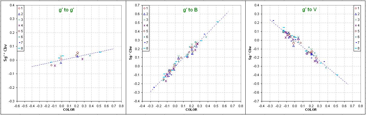
Figure 08. Comparison of star color sensitivities for the three
ways to use g' measurements.
Referring back to Fig. 01 note that the effective wavelength of the g'
passband is between B and V's effective wavelengths. It is therefore no
surprise that the color sensitivities for using g' to derive B and V are
large and of opposite sign. It is also to be expected that the g' to g'
slope is small. The fact that it has a slightly positive slope implies that
my telescope system's g' response function (related to transmission function)
is slightly blue-ward of the standard system's response function.
Repeat of Fig. 4.
Returning to Fig. 04, repeated above, some of the other cells can be explained.
The model fit is:
g'-mag = 19.918 - 2.5 ×
LOG ( Flux(g') / g ) - 0.207 × AirMass + 0.118 × StarColor
(6)
Notice that with a solution for the two constants in green (Zg' and Sg')
everything is availalbe to compute g'-mag from a g' flux measurement of
an unknown target star except StarColor! Note the definitions for StarColor
in the above figure.It can be calculated from either g'-r' or B-V. We can't
get the target star's color from g'-r' because it is unknown at this stage
of analysis and this is part of what we're trying to determine. We also can't
get StarColor from B-V for the same reason. One possible solution is to
note that StarColor doesn't matter much because Sg' is small and almost
any first guess, such as zero (the median star color for the set of 1264
Landolt stars, as I define StarColor), and proceed to caclulate r' using
a spreadsheet page identical in structure to that for g', and use the same
argument in deriving a first estimate for r'; the first estimates of g'
and r' can be used as input to both the g' and r' pages to arrive at a first
iteration solution for g' and r' (and StarColor based on g'-r'). This solution
works well and in my experience in similar situations only two or there iterations
are needed to achieve a stable solution. A second solution is to use the
target star's J and K magnitudes to solve for B and V, which is just as good
a path for deriving StarColor. I prefer the JK conversions to BVRcIc published
by Brian Warner and Alan Harris (2007). Almost all stars brighter than 15th
V-mag have JHK mags so usually this method for estimating StarColor is available.
A spreadsheet page for r' is used in exactly the same was as the one for
g'. Following are plots from this page.
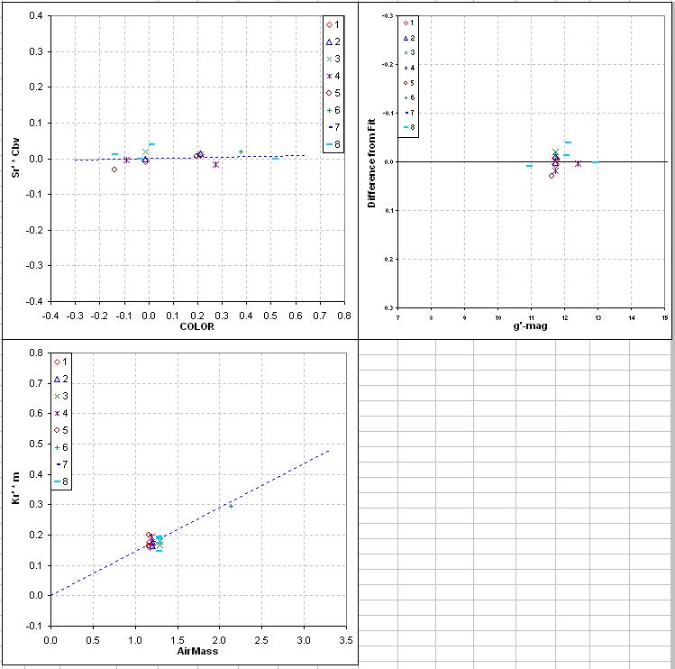
Figure 09. Counterpart to Fig. 4 except for g' flux measurements
used to predict g' magnitudes. The slope for the extinction plot (lower-left
plot) corresponds to atmospheric extinction at r'-band.
Notice the almost zero slope for the r' star color sensitivity parameter
Sr'. Apparently my telescope system's equivalent response wavelength for
r' is close to that for the standard r' system. This means that I can solve
for r' for an unknown target star without knowing anything about its StarColor.
The extinction plot for r' has a poorly-defined slope. As with g', we can
get a much better constrained extinction slope from a spreadsheet page that
compares r' fluxes to known Rc magnitudes. The 3-plot set for r' to Rc is
shown next.
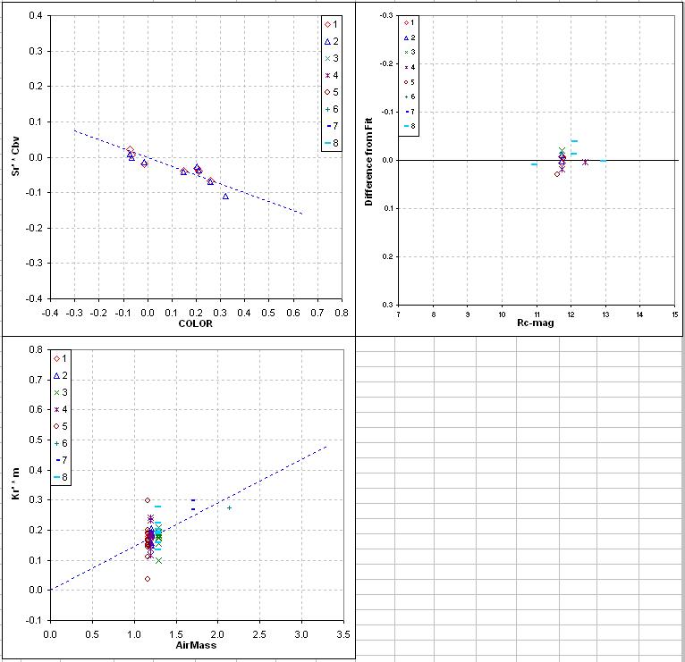
Figure 10. Counterpart to Fig. 4 except for r' measurements related
to calibration star Rc magnitudes. The slope for the extinction plot (lower-left
plot) corresponds to atmospheric extinction at r'-band.
The extinction plot doesn't have as many high airmass samples as we'd like,
which is an oversight on my observing session planning. There are fewer
Rc stars than B or V stars because Landolt's list contains fewer stars with
calibrated Rc and Ic than B and V. A consensus zenith extinction for r'-band
is 0.145 [mag/airmass]. This is close to my observing site's historical Rc-band
extinction of 0.16 [mag/airmass]. Later in the spreadsheet analysis we'll
have another opportunity to refine Kr'.
At this stage of analysis we are able to obtain good estimates for StarColor
from the g' and r' solutions, which can be iterated to stability. We also
have shown how to solve for B, V and Rc magnitudes. Unknown target stars
can be used with these several basic magnitude equations to solve for
all of the following: B, V, Rc, g' and r'.
What about i' and Ic? The same concepts apply, and I'll merely show figures
for this observing sessions solutions. Descriptions won't be necessary.
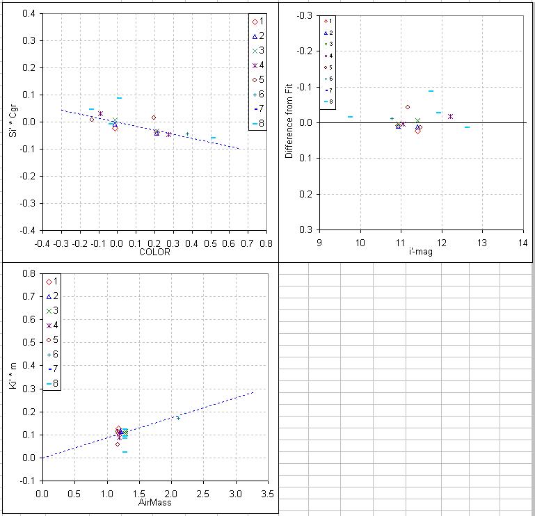
Figure 11. i' flux measurements to i' magnitude plots.
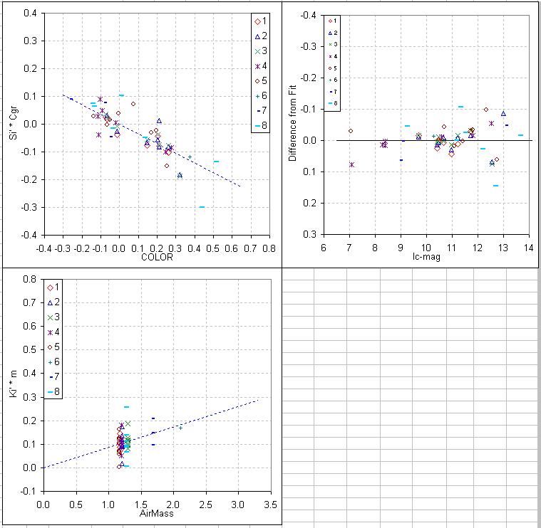
Figure 12. i' flux measurements to Ic magnitude plots.
The final set of basic magnitude equations that resulted from this spreadsheet
analysis is given below.
Recall the following notation: B(g') means a B-band magnitude derived from
g' star flux measurements, g' means g' magnitudes derived from g' flux measurements,
etc.
The stated RMS accuracies are simply the RMS of residuals of Landolt or
Flagstaff SDSS star magnitudes from the equation fits. The median RMS accuracy
is 0.028 magnitude, which is typical for all-sky observing sessions
with amateur hardware and software. Arne Henden probably achieves something
like 0.010 to 0.020 mag routinely, using professional hardware and software.
Arno Landolt achieves ~ 0.001 mag accuracies after averaging many observing
sessions using a photomultiplier tube at professional observatories.
4. UNKNOWN
STAR FIELD PLOTS
An unknown star field was observed at air mass values similar to most of
the Landolt and Flagstaff SDSS star field air masses, and the following
figures were obtained after iterating the g' and r' provisional magnitude
values to a stable solution. Note that for all these fits there was no freedom
to adjust Z or S or K' because these coefficients were determined for each
filter band using Landolt and SDSS stars. The only free parameters for the
unknown star fields are the magnitudes which we are trying to establish.
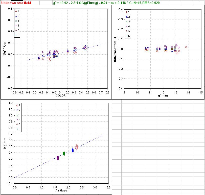
Figure 13. Unknown star field iterated solution for g' magnitudes
from g' flux measurements for 4 observing sequences.
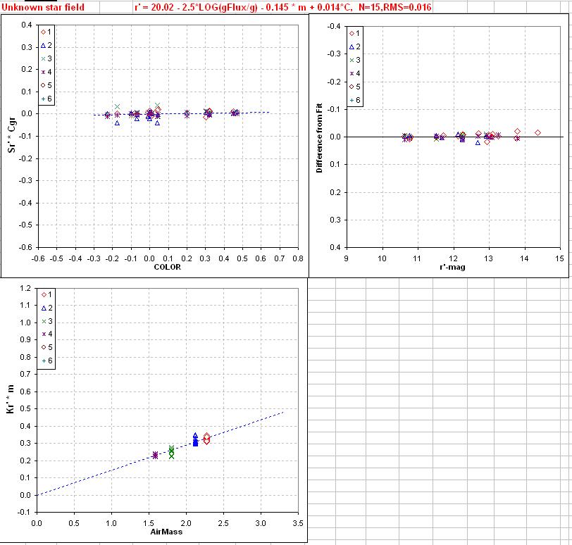
Figure 14. Unknown star field iterated solution for r' magnitudes
from r' flux measurements for 4 observing sequences.
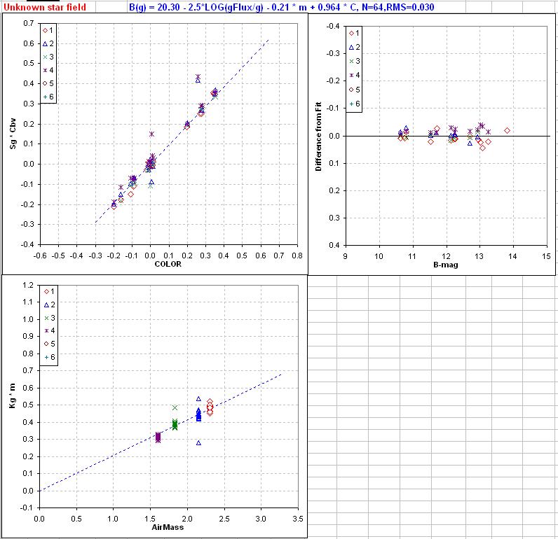
Figure 15. Unknown star field iterated solution for B magnitudes
from g' flux measurements for 4 observing sequences.
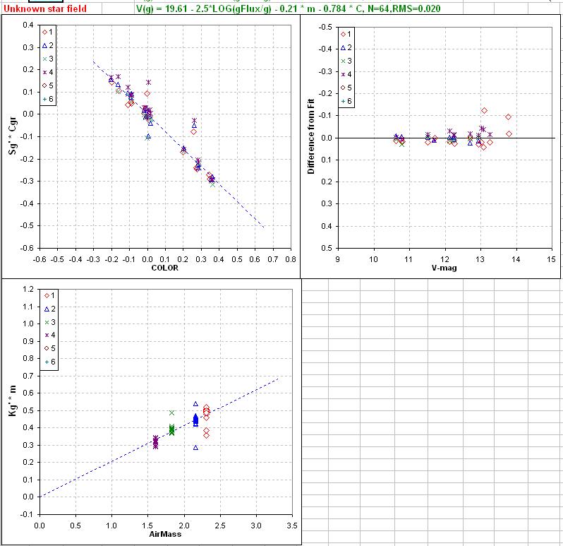
Figure 16. Unknown star field iterated solution for V magnitudes
from g' flux measurements for 4 observing sequences.
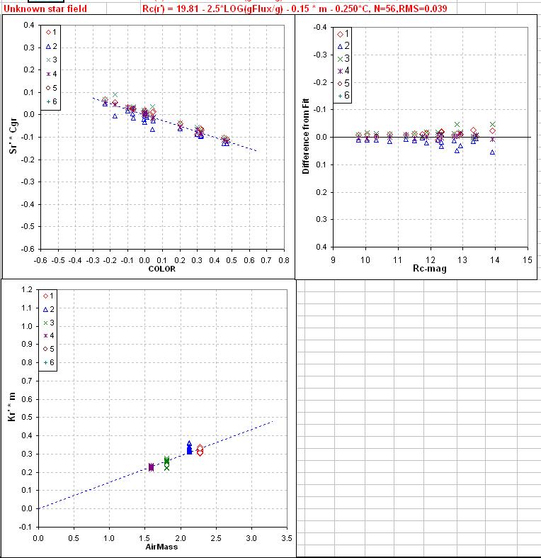
Figure 17. Unknown star field iterated solution for Rc magnitudes
from r' flux measurements for 4 observing sequences.
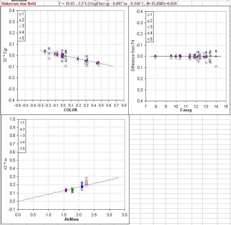
Figure 18. Unknown star field iterated solution for i' magnitudes
from i' flux measurements for 4 observing sequences.
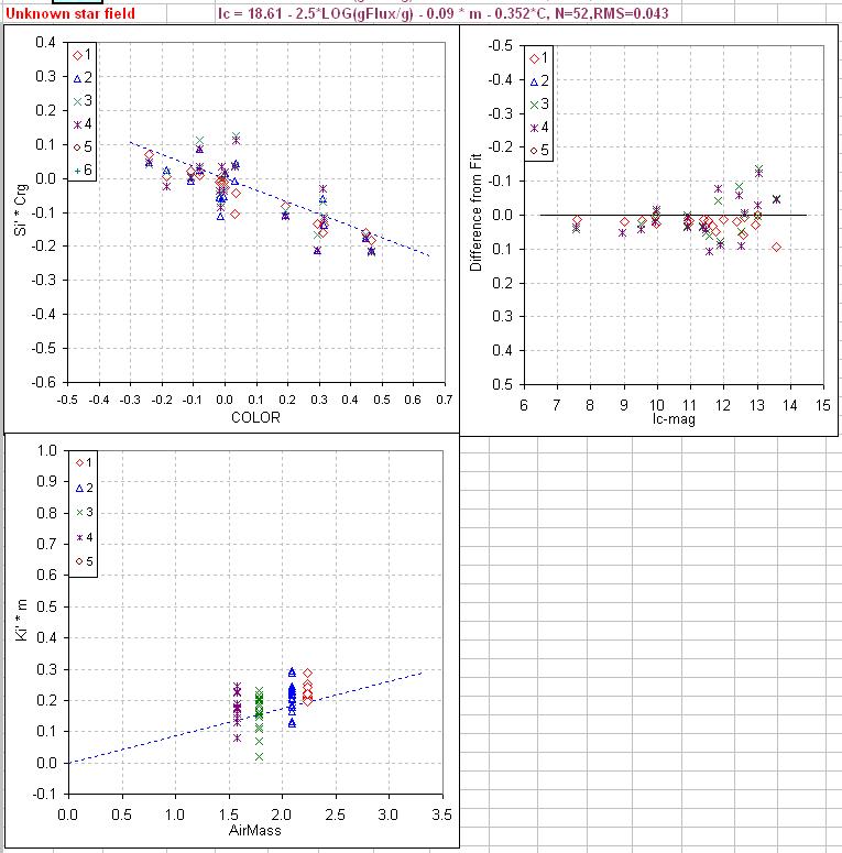
Figure 19. Unknown star field iterated solution for Ic magnitudes
from i' flux measurements for 4 observing sequences.
5. UNKNOWN TARGET STAR MAGNITUDES
The procedure I describe for deriving magnitudes from flux readings has
yielded the following results for the target:
g' = 12.450 ± 0.020
r' = 11.937 ± 0.016
i' = 11.811 ± 0.028
B = 12.839 ± 0.023
V = 12.135 ± 0.031
Rc = 11.750 ± 0.039
Ic = 11.390 ± 0.043
The stated SEs are merely the RMS residuals of all Landolt and Flagstaff
SDSS stars from the "basic photometry equation" model fits.
6. REALITY CHECKS
No result should be accepted without subjecting it to "reality checks." Fortunately,
there are several such checks that can be made of the 7 magnitudes for the
target star. Since the 17 nearby stars share the same systematic errors with
the target it is possible to indirectly check the target star magnitudes
by checking the consistency of these nearby star magnitudes with expectations.
RealityCheck #1
Section 4 has plots of unknown star magnitudes versus a model for each filter
band that was based on the Landolt and SDSS stars. The only fitting done
for the unknowns stars was an iteration sequence of their g'r'i'BVRcIc magnitudes
using the fixed "basic magnitude equation" model parameters. If the model
parameters are accurate it should be possible to find a good solution
for the unknown star field magnitudes. This indeed is the case, as can be
seen by visual inspection of the figures in Section 4. This constitutes a
"reality check" on the procedures implemented in the spreadsheet and provides
confidence that maybe the target magnitudes are accurate.
Reality Check #2
Another "reality check" can be made by plotting the derived magnitudes
for the target and 17 nearby stars on color-color scatter diagrams that
include the Landolt list of 1264 stars.
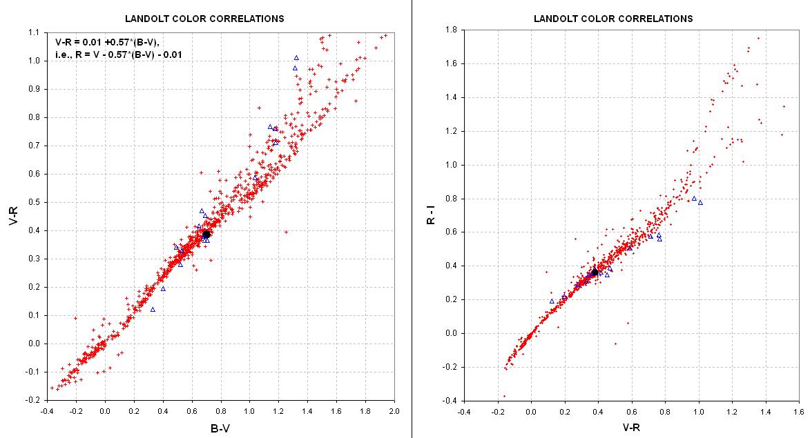
Figure 20. Color-color scatter diagram showing how the magnitude
solutions for the target star (solid black circle) and nearby 17 nearby
stars (open blue triangels) compare with the 1264 Landolt stars.
Some of the nearby stars are quite faint, accounting for most of the large
departures from the consensus locus of Landolt color-colors. Overall, the
pattern of unknown star field colors is consistent with normal star fields
that have been accurately calibrated, which constitutes another reality check
for the target magnitudes.
Reality Check #3
A third reality check is to convert the g'r'i' magnitudes to BVRcIc using
conversion equations dervied by professionals and compare them with the
magnitudes derived from direct solutions, i.e., solutions of BVRcIc based
on g'r'i' flux readings. Smith et al, 2002 give the following:
B = g' + 0.47 (g'-r') + 0.17
V = g' - 0.55 (g'-r') - 0.03
Rc = V - 0.59 (g'-r') - 0.11
Ic = Rc - 1.00 (r'-i') - 0.21
Using these equations for the target star yield the following:
B = 12.853 ± 0.023 vs 12.839 ± 0.023 from
g' to B directly (difference = +0.014 ± 0.032)
V = 12.150 ± 0.024 vs 12.135 ± 0.031 from g'
to V directly (difference = +0.015 ± 0.039)
Rc = 11.749 ± 0.029 vs 11.750 ± 0.039 from r' to Rc
directly (difference = -0.001 ± 0.048)
Ic = 11.392 ± 0.043 vs 11.390 ± 0.043 from i' to Ic
directly (difference = +0.002 ± 0.061)
Both ways of deriving BVRcIc agree, so the third reality check is passed.
Reality Check #4
Finally, a fourth "reality check" can be made using JK-based magnitudes
for BVRcIc. For the target we have:
J = 10.820, K = 10.421,
and using the Warner and Harris (2007) conversions yields:
B = 12.768 ± 0.080 vs 12.839 ± 0.023 from
g' to B directly (difference = -0.071 ± 0.083)
V = 12.095 ± 0.050 vs 12.135 ± 0.031 from g'
to V directly (difference = -0.040 ± 0.059)
Rc = 11.713 ± 0.040 vs 11.750 ± 0.039 from r' to Rc
directly (difference = -0.037 ± 0.056)
Ic = 11.345 ± 0.035 vs 11.390 ± 0.043 from i' to Ic
directly (difference = -0.045 ± 0.055)
In every case the difference is less than the estimated SE, so the BVRcIc
magnitudes derived directly from g', r' and i' flux measurements are compatible
with JK-based magnitudes.
Reality Check #5
Figure 20 is a check of just 3 star colors (B-V, V-I and R-I) involving 4
filter bands. What about the other 3 filter bands? One way of representing
them is to compare the 7 band "spectrum" of the unknown target star with
Landolt/SDSS stars. To do this it will be helpful to offset all stars so
that they have the same value at a specific wavelength, such as V-band. The
following figure shows the first 11 Landolt/SDSS star magnitudes plotted
at the filter's effective wavelength. The red stars exhibit a smooth trace,
while the blue stars show irregularities longward of V-band. The progression
of shapes appear to be correlated with the "color" B-Ic (which is how they
are ordered). If the target star's 7 magnitude solution is accurate it is
likely to resemble one of these Landolt/SDSS stars. Does it?
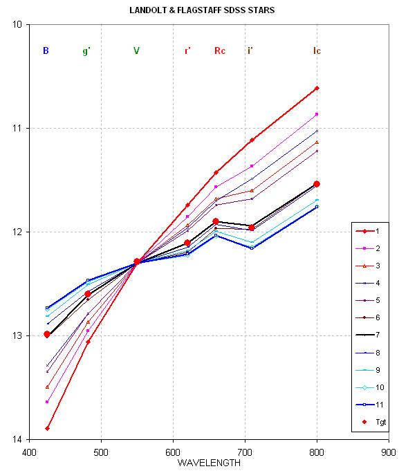
Figure 21. Broadband "spectrae" of Landolt/SDSS stars, offset so
that V = 12.3, ordred by blueness. The unknown target star (lage red circles)
most resembles Landolt/SDSS star #7.
The target star most resembles Landolt/SDSS star #7, which is plotted with
a thick black trace. The RMS difference between the target star's 7 magnitudes
and those for Landolt/SDSS #7 is 0.014 magnitude. The resemblance is quite
good! The 5th reality check is therefore a success.
Conclusion
I never said this was easy, or quick! Lot's of manual effort is required
to arrive at the results illustrated here. The professionals have program
"pipelines" for achieving the same result, and probably relying on equivalent
procedures based on the same basic concepts employed here. I doubt that
a pipeline would work for amateur observations because amateur hardware
has many handicaps the professionals never have to worry about. The measurements
reported here were made with an 11-inch telescope and an old SBIG CCD.
It is important to adopt observing and analysis techniques tailored to your
hardware and observing site. Most amateurs wanting to try all-sky photometry
will probably have similar limitations, which means they probably will have
to employ analysis techniques similar to those illustrated on this web page.
Good luck!
Related Web Page Links
AAVSO photometry manual: http://www.aavso.org/observing/programs/ccd/manual/4.shtml#2
Lou Cohen's 2003 tutorial: http://www.aavso.org/observing/programs/ccd/ccdcoeff.pdf
Priscilla Benson's (1990's) CCD transformation equations
tutorial: http://www.aavso.org/observing/programs/ccd/benson.pdf
Bruce Gary's CD Transformation Equations derived from basic princples: http://reductionism.net.seanic.net/CCD_TE/cte.html
Bruce Gary's
All-Sky Photometry for Dummies: http://brucegary.net/dummies/x.htm
Bruce Gary's All-Sky Photometry
for Smarties - v1.0: http://brucegary.net/photometry/x.htm
Bruce Gary's All-Sky Photometry for
Smarties - v2.0: http://brucegary.net/ASX/x.htm
Bruce Gary's Differential Alternative Equations http://brucegary.net/DifferentialPhotometry/dp.htm
Bruce Gary's Astrophotos home page http://reductionism.net.seanic.net/brucelgary/AstroPhotos/x.htm
____________________________________________________________________
WebMaster: Bruce
L. Gary. Nothing
on this web page is copyrighted. This site opened:
2009.10.03 Last Update: 2009.10.04