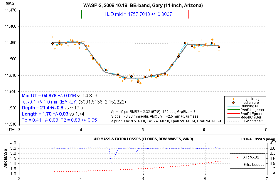
Light curve obtained by the webmaster.
This web page is intended for use by "students" for processing images of
an exoplanet transit in order to produce a transit light curve. The goal is
to achieve a result somewhat similar to the following.
Light curve obtained by the webmaster.
The following links are for downloading raw image files, flat field and
dark frame calibration files and a bias image file, all of which can be used
for creating a transit light curve. In addition I have included a "master"
image file that can be used for star-aligning the calibrated image files (although
it would be good practice to create this file by median combining a few of
the calibrated image files). All files are zip-versions. The raw image sets
are in groups to keep download times manageable. Most raw image groups are
~15 Mb in size.
Links to Files
Dark
Frame Image
FlatFieldImage
Bias Image
Master Image
Raw Image Set #01 (first
10 images)
Raw Image Set #02 (next
10 images)
Raw Image Set #03 (next
10 images)
Raw Image Set #04 (next
10 images)
Raw Image Set #05 (next
10 images)
Raw Image Set #06 (next
10 images)
Raw Image Set #07 (next
10 images)
Raw Image Set #08 (last
5 images)
The image scale is 0.74 "arc/pixel and the FOV is 18.9 x 12.6 'arc. North
is up, east to the left. Exposure times are 120 seconds. The FOV center coordinates
are RA = 06:02:30, DE = +06 21:46.
Some Hints
I suggest the following procedure (note chapters treating these subjects in my book free-download book Exoplanet Observing for Amateurs):
Calibrate all raw images using the dark field, flat
frame and bias frame images. Chapters 12.
Align all calibrated images using the master image (extra
credit for making your own master image). Chapter 12.
Add the artificial star to the upper-left corner of each
image. Chapter 12.
Use MaxIm DL's photometry tool, selecting the Object
(WASP-2), reference star (the artificial star) and many "Check Stars" (intended
for use as reference stars in the spreadsheet). Chapter 12.
When saving CSV-files (the objective of the photometry
tool) use a selection of signal aperture radii. The rule of thumb is to prefer
a radius that is ~3 times the FWHM [pixels]. Chapter 10.
Import a CSV-file to a spreadsheet. This is where your
creativity will be tested. Think about the concepts that must be dealt with,
such as extinction, use of stable reference stars, rejecting noisy (outlier)
data, etc. These issues are treated in my Chapter 13.
Here's an example of what you could see while using MaxIm DL's photometry
tool (after selecting Obj, Ref and Chk):
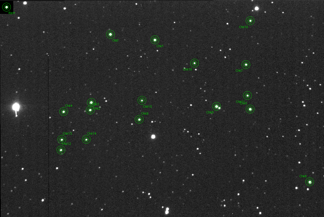
Photometry tool display after selecting WASP-2 as the Object ("Obj1"),
the artificial star as a Reference ("Ref1") and (in this case) 16 stars as
check ("Chk1" etc).
Good luck!
Additional Notes
There are two uses for the artificial star: 1) to permit determination
of extinction coefficient, and 2) to permit calculation of "extra losses"
(clouds, smeared PSF due to bad seeing or tracking errors). It's actually
optional to use an artificial star; if it's not used then simply specify the
many star to be used for reference as "Reference."
This image set contains many problems found in a typical observing session.
The autoguider lost track at Image #057, and it's a pathetic-looking image.
I left it in the image set in order to show that it has no degrading effect
when the spreadsheet is used to reject outliers. Many images are not sharp,
due to imperfect tracking. Again, this has minimal effect on the final LC
provided the spreadsheet is used carefully. You'll note that the dark calibration
frame was made with a different exposure (& temperature) than the image
frames, so there are artifacts caused by an imperfect calibration scaling
(most noticeable as a dark vertical line on the left). Also note that Chk8
has a sky background annulus with a bright star inside. This shouldn't matter
because MaxIm DL's photometry tool has a sophisticated algorithm for recognizing
which pixels are affected and not using them. The two brightest stars were
"saturated" (max counts > 50,000 for my CCD), so I didn't use them for
reference. It's generally not a good idea to use stars near the corners for
reference but since the flat field appeared to be doing a good job I took
a chance with "Chk6" and "Chk10." I used an autoguider (the AO-7, with a tip/tilt
mirror) to keep the star field fixed with respect to the pixel field. This
is most successful when the polar axis is aligned accurately, to prevent image
rotation (about the autoguider star); I always strive for <0.1 degree.
When autoguiding is lost I re-center carefully so the same autoguide star
is at the same x,y location on the autoguider chip. These images were made
with a blue-clocking filter, which passes everything longward of ~480 nm.
A clear filter would have worked just a well. I've become an advocate of "clear"
provided a spreadsheet is used to identify & reject for use candidate
reference stars that show them to have a noticeable air mass curvature systematic
effect.
____________________________________________________________________
WebMaster: B.
Gary.
Nothing on this web
page is copyrighted. This site opened: 2009.01.05. Last Update: 2009.02.24