FILTER PLAYOFF OBSERVATIONS

Summary of Results

Observations were made of CoRoT-3 on 2009.09.14 using filters CBB, NIR, V, Rc and i’ rotated into place in alternation. Exposure times were set in a way that led to similar total flux (and SNR) for the target for each filter. A standard procedure was used for image processing and spreadsheet light curve optimization for each filter. Since for this 5-hour observing session there was no transit the data were fitted using a simple model with three free parameters (offset, slope and air mass curvature). RMS departure from the best model fit was used to assess measurement quality. Since exposure times ranged from 5 seconds to 32 seconds a “figure of merit” was calculated that endeavors to predict the RMS quality of what would have been measured if each filter were used exclusively during the observing session. The figure of merit is proportional to “information rate” (proportional to the inverse square-root of the predicted RMS off a model light curve) using exposure times of 48 seconds and download and settle times totaling 12 seconds (which are typical observing settings for amateur telescopes observing typical exoplanet stars). Such a figure of merit can be described as the speed with which a specific precision can be achieved. The results of these calculations show the following “speed for reaching a precision goal”, presented in order of the fastest (and normalized to the slowest filter): CBB (6.3), Rc (2.9), NIR (1.7), i’ (1.3) and V (1.0). For this observing situation the CBB filter was about 6 times better than the V-band filter. Since CoRoT-3 is fainter than the typical exoplanet star the same set of 500 images was re-processed with a brighter star assigned to the role of exoplanet. For a “make believe” exoplanet star with V = 11.7, similar to the median for the list of 46 BTEs, the following figure of merits were determined: CBB (8.1), NIR (5.4), Rc (5.1), I’ (4.6) and V (1.). When an even brighter star was assigned the exoplanet star role (V = 10.2) the results were essentially the same: i’ (8.1), NIR (6.8), CBB (6.2), Rc (5.4) and V (1.0).

Introduction

The observations reported here were designed to determine which filter produces the best quality light curves for typical exoplanet observing conditions using amateur hardware and software. I use my Celestron 11-inch (CPC 1100) telescope with a focal reducer placed in front of the CFW/CCD. The CCD is a SBIG ST-8XE (KAF 1602E chip). Autoguiding is performed using the second CCD chip. The CFW contains the following filters, all of which are used in this evaluation: CBB, NIR, V, Rc and i’ (where CBB is a clear filter with blue blocking at ~ 480 nm, NIR is a long pass filter with turn-on at 710 nm, V is Johnson V-band, Rc is a Cousins R-band and i’ is SDSS i-band). Although additional observing sessions may be used to verify the results reported here the following description of the first observing session, on 2009.09.14, shall serve to illustrate the protocol and analysis procedures for all of them.

Observation Protocol

The observing session was 4 hours long (after which the dome’s low-elevation opening obstructed observations). Observations started at air mass 1.2 and data for air mass > 4.5 were not used. CoRoT-3 was observed under out-of-transit conditions. This enabled the measured magnitudes to be fitted using a simple light curve (LC) model with only three free parameters (offset, slope and air mass curvature). It was decided to employ exposure times that produced approximately the same flux for the target star (CoROT-3) for each filter (Arne’s suggestion). This led to greatly different exposure times due to the large range of filter throughputs. Filter throughputs for all the filters I use are listed in the following table, and the exposure times used for this “filter playoff” observing session are included. For the chosen exposure times the star fluxes for the target were approximately the same and so were the SNR’s (although SNRs should differ because sky background levels differ with wavelength).

Filter Throughput (at airmass 1.2) and Exposure Times

CLR 100%

CBB 92% 5 sec

NIR 37% 16 sec

B 6%

V 19% 32 sec

R 36% 14 sec

I 22%

g’ 26%

r’ 48%

i’ 37% 16 sec

z’ 9%

Images were made in the following sequence: NIR, V, Rc, i’ and CBB. Exactly 100 cycles of this sequence were made (prior to the dome obstruction problem), so there are 100 images with each of these 5 filters. Autoguiding was used to maintain the star field fixed to the CCD pixel field (although some wander did occur). Master flats were made on the same night of these observations for each filter using the twilight sky (and a diffuser over the telescope aperture). A master dark frame was made at the end of the target observations (at the same CCD temperature as the target observations). A bias frame was used from a previous observing session. Focus settings were automatically adjusted to compensate for telescope tube temperature changes. Measures were taken so that all images had the same sharpness (FWHM typically 4.5 pixels). All observing was controlled by MaxIm DL (MDL).

MDL was also used for image calibration and measurement. Calibration consisted of bias, dark and flat field corrections. Hot pixels were removed from each image (25% was determined to be “safe” because it didn’t change a star’s maximum count for many tests of sharp images). Star alignment was made for all images for a filter group. MDL was then used to perform photometric measurements of the target star (CoRoT-3), the artificial star (flux the same for all images) and 27 nearby bright (unsaturated) stars. CSV files were recorded for measurements made with a selection of photometry aperture radii. It is well known that the optimum aperture size depends on SNR. Faint asteroids provide the best rotation LCs for a photometry aperture radius, r, of about 1.4 x FWHM. Bright stars produce the best LCs for r about 3 x FWHM. CoRoT-3 is of intermediate brightness for the present choice of exposure times (SNR ~ 40) so the range of photometry apertures employed was from ~1.8 to 3 x FWHM.

A spreadsheet was used for the rest of the analysis. Star magnitudes were converted to flux, and these were added for all 27 non-target stars in order to solve for atmospheric extinction. It was found that extinction ranged from 0.065 mag/airmass (NIR) to 0.160 mag/airmass (V-band). A search was made for which subset of the 27 stars provided the lowest RMS noise for the target. This RMS noise was calculated by comparing each target star magnitude with the median of its 8 closest neighbors, and a standard deviation of all such differences (with a small correction for the fact that 8 isn’t infinity) was used to establish an RMS for the observing session. The next step was to model-fit the target magnitudes using as a criterion the lowest RMS deviation from the model, RMSmodel. When a good model fit was found a search was made of reference star sub-sets that produced the lowest RMS deviation from the model. This step usually did not lead to many changes in reference star selection (change would occur if systematic effects differed among the 27 candidate reference stars). If a large improvement in fitting the model was achieved by changing the reference star sub-set then another iteration was performed: model fit for minimum RMSmodel, search for a better reference star subset (that reduces RMSmodel). It is rare to have to iterate like this more than once. I view the final model and reference star subset to be a “global minimum” solution.

Observational Results

The next figure is a “solution” for CBB.

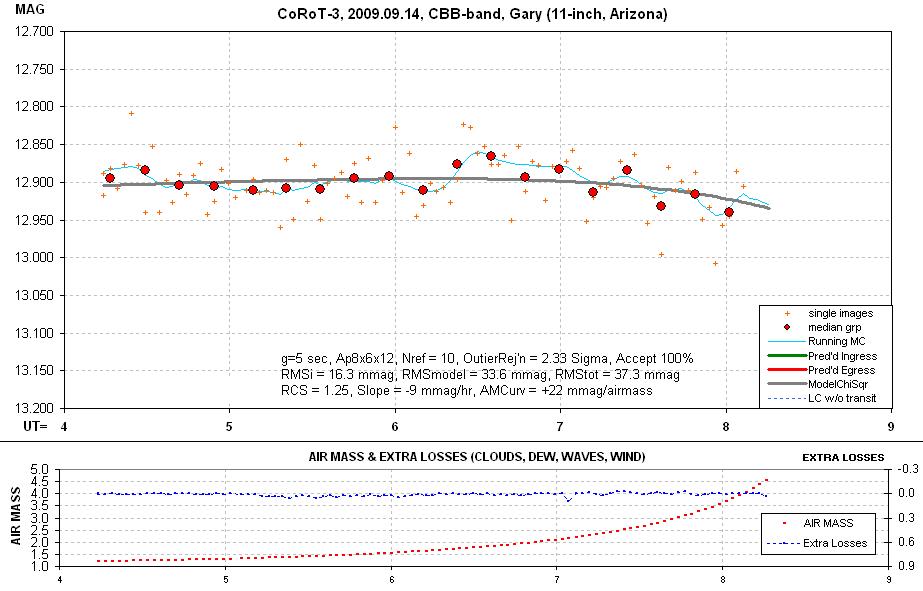
Figure H01. Example of a LC solution. The filter is CBB and exposures were 5 seconds.

The other filters produced similar looking light curves. The target is bluer than average (B-V = +0.91), so most of the references stars must be redder. Notice that air mass exceeds 3.0 during the last 40 minutes, and this, combined with the difference in color of the target and references stars, must cause the model fit to require an “air mass curvature” component.

The next table summarizes the measurements for each filter image set. The first row (below filter names) is “throughput” – or percentage of light from a typical star that reaches the CCD when a filter that is in the optical path compared to the amount of light reaching the CCD when no filter is in place. The second row is the median FWHM of the images. The third row shows the photometry aperture radius that produced the best result. By best result is meant the smallest RMS departure from the LC model fit (where all of the following parameters were optimized: sub-set of candidate reference stars used for reference and model offset, slope and airmass curvature). The next row shows atmospheric extinction. The next row shows RMSi, which is the RMS of measurements with respect to the median of the 8 nearest neighbors. This noise is for a short timescale, and if systematics vary slowly they will not affect RMSi. Next is RMSmodel, which is the RMS deviation of differences with the best fitting model LC. This RMS can be thought of as the orthogonal sum of RMSi and RMSsys (systematics). Therefore, by orthogonally subtracting RMSi from RMSmodel we arrive at RMSsys, shown in the next row. Exposure time, g, is shown in the next row. Info/image is “information per image”, calculated from the inverse square of RMSmodel. The next row converts RMSmodel and exposure time to “Precision per minute of observing time” under the assumption that one exposure is made each minute with an exposure time of 48 seconds (which allows 8 seconds for download and 4 seconds for autoguider re-acquisition). This row is calculated by multiplying RMSmodel by the square-root of g/48. Finally, a Figure of Merit is calculated by multiplying a constant by the inverse square of the previous row. The constant is chosen so that the V-band filter has a Figure of Merit equal to one. This Figure of Merit can be viewed as the speed with which a specific precision can be achieved. For example, if a precision of 27.6 mmag per minute of observing time is chosen as the goal, then using the V-band filter this level of precision can be achieved in 1 minute. If the Rc-band filter were used this level of precision could be achieved 2.93 times faster (or 20 seconds, neglecting for now that short exposure times incur a duty cycle penalty). For the CBB filter a specific level of precision can be achieved 6.3 times faster than if the V-band filter were used.

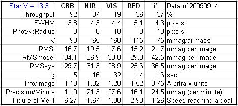
Figure H02. Summary of filter playoff results for the CoRoT-3 (V = 13.3).

There are some instructive things to notice about this table. The values of RMSi should decrease with increasing exposure time, according to 1/sqrt(g), if we’re in the “faint star” domain – where stochastic noise (thermal, sky background, etc) is dominant. The values for RMSsys, however, should not change with exposure time since they are a component of systematics that presumably varies slowly with time (as the star field slowly moves over the CCD field, for example) and some components of systematics will be approximately the same for each filter.

RMSi consists of two major components: Poisson noise and scintillation noise. It is always interesting to keep track of the importance of scintillation noise in order to know how to fine-tune observing strategy. Although the level of scintillation can change greatly from night to night, or even on hour timescales, it’s worth asking what a typical scintillation level should be for the observing conditions of this case study. According to Dravins et al (1998):

where sigma is RMS fluctuation (fractional intensity), D is telescope diameter (cm), sec(Z) is air mass, h is observing site altitude (meters) and g is exposure time (seconds). All observations reported here have the same D and h, so this equation becomes:

Sigma [mmag] = 5.8 * AirMass^1.75 / sqrt(g)

The highest scintillation level is predicted for CBB-band near the end of the observing session; during the last 40 minutes the scintillation level is predicted to be ~ 23 mmag. Inspection of the RMSi(t) plot shows an increase at this time, being ~38 mmag (instead of 32 mmag before then). These two RMSi values are consistent with the predicted scintillation increase. For the other filters and exposure times predicted scintillation was never significant.

It is interesting to note the relation between “Precision per Minute” and filter throughput.

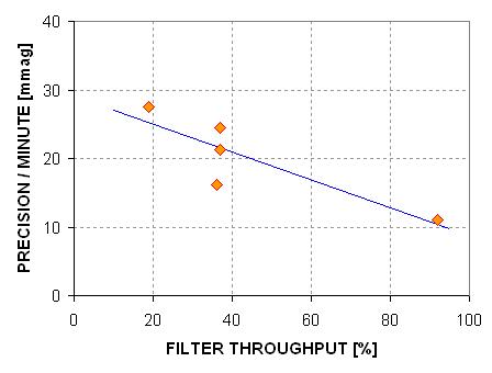
Figure H03. Precision/Minute versus filter throughput (13.3 magnitude star and 11-inch aperture).

The message of this plot is “The greater the filter throughput the better the precision!” This may simply be a consequence of observing a faint target (SNR ~ 40 for all filters). This result suggests that optimum filter choice may depend on target brightness, and the results so far are what we can expect for the faint regime. It is therefore not surprising that for this example the Figure of Merit is correlated with filter throughput. Just because the CBB filter is optimum for faint exoplanet stars doesn’t mean it will be optimum for bright exoplanet stars.

Fortunately, the set of images used in the analysis so far can be used to evaluate Figure of Merit for a brighter star. This can be done by simply selecting a brighter star for treatment as the “target.” That’s the goal of the next section.

Average BTE Brightness Target Star Analysis

The following figure shows two other stars that can serve as surrogate exoplanet stars in OOT mode available for use to evaluate Figure of Merit versus star brightness.

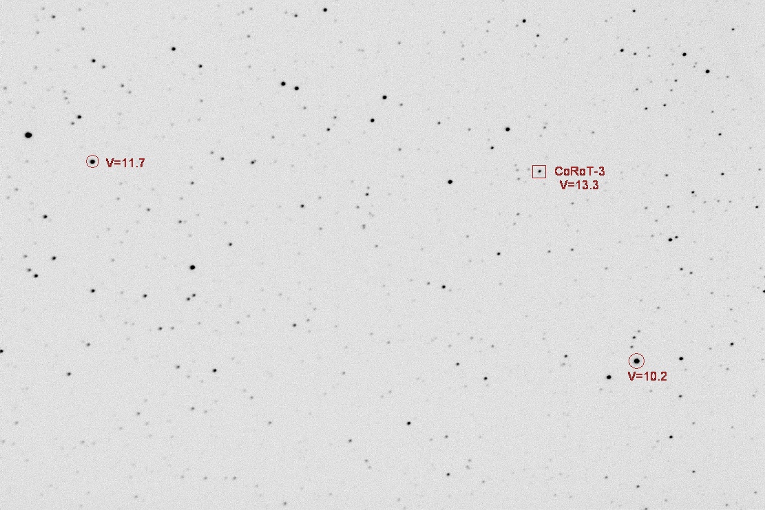
Figure H04. CoRoT-3 FOV, 22x14 ‘arc, showing two stars brighter than CoRoT-3.

The star labeled V=11.7 is 1.6 magnitudes brighter than CoROT-3 and is also close to the median brightness of the list of 46 known BTEs. It will be used to determine filter performance in a way analogous to what was done in the previous section.

The same procedure used for CoRoT-3 was used with the V-mag = 11.7 star. As expected the LC quality for this brighter star is better than for the 13.3 magnitude exoplanet star. The next figure is the LC using the NIR filter.

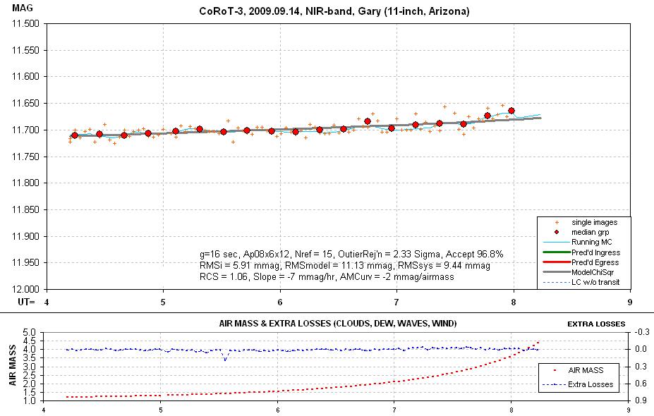
Figure H05. NIR filter LC for the V-mag 11.7 star.

The following figure summarizes results for this star for the 5 filters.

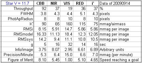
Figure H06. Summary of observations of a star with V = 11.7, similar to typical BTE.

The highest Figure of Merit is obtained using the CBB filter, but the NIR, Rc and i’ filters are all a close second. The V-band filter is the slowest choice for achieving useable LCs.

Precision per Minute is not as strongly correlated with filter throughput as it is for the fainter star, as the next figure shows.

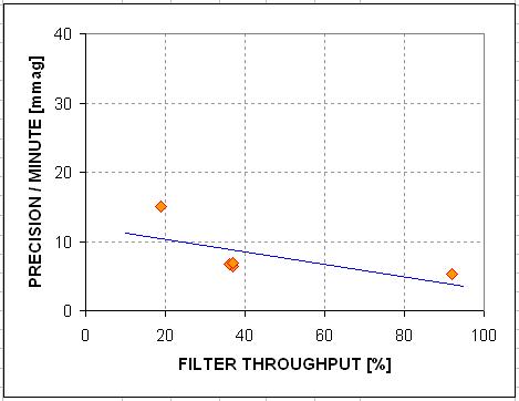
Figure H07. Precision performance versus filter throughput for the V = 11.7 star.

Scintillation is predicted to be more important for the brighter star simply because other stochastic noise levels are lower (whereas scintillation level is the same for all stars, regardless of their brightness.) The scintillation levels for each filter will be the same as calculated above, for fainter CoRoT-3. As stated above, the highest scintillation is expected for the CBB images, with a low of 3.6 mmag for the first few hours and an average of ~23 mmag during the last 40 minutes. A plot of RMSi(t) shows a rise from ~12 mmag during the first few hours to ~25 mmag near the end of the observing session. This could be explained if scintillation near the end was ~22 mmag, which is close to what is expected from the Dravins et al (1998) scintillation model. Scintillation levels for V-band ranged from 1.4 mmag to 9.2 mmag, and these are small enough to have only small effects on the observing session averages.

For given levels of noise and scintillation, if we ignore the effect of duty cycle on exposure time, longer exposure times don’t reduce the effect of scintillation when considering “information rate” – or Precision per Minute of observing time. In other words, the average of 10 short exposures will have the same level of scintillation noise as one exposure 10 times as long. This concept is commonly understood for other stochastic noise levels (such as thermal noise, sky background noise, etc), but when the issue is scintillation there is a tendency to forget the concept and mistakenly recommend long exposures to reduce scintillation.

Brighter Than Average BTE Target Star Analysis

Finally, let’s consider a star brighter than most exoplanets to see if CBB continues to outperform the other filters. The V = 10.2 star, shown in Fig. A04, has been processed using the same procedure used for the two fainter stars. The LC performances for the i’ and V filters are shown in the next two figures.

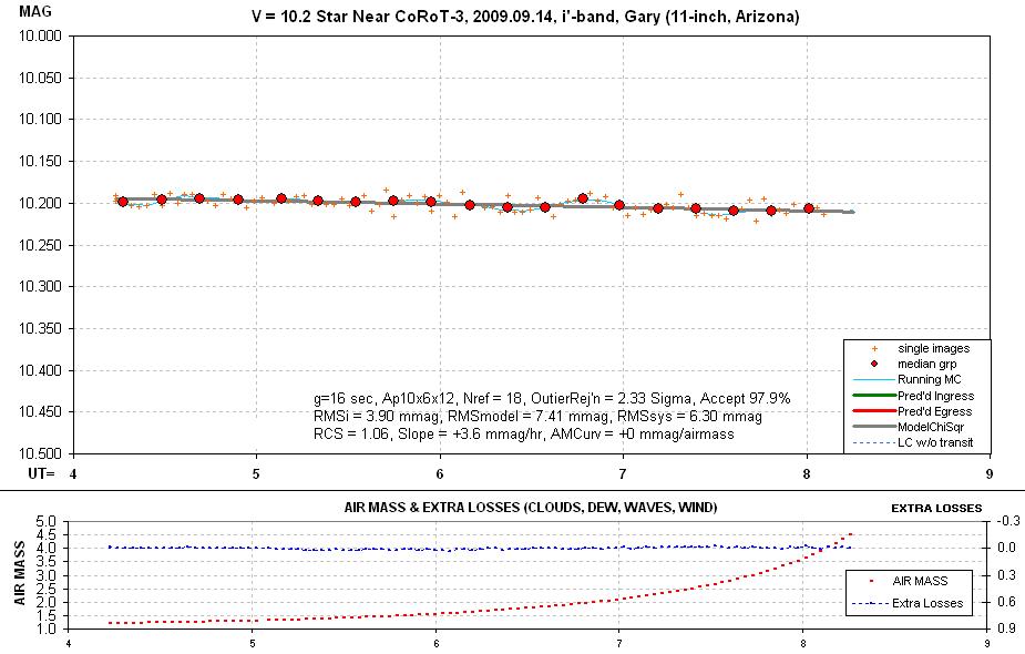
Figure H08. i’-band light curve for the V = 10.2 star.

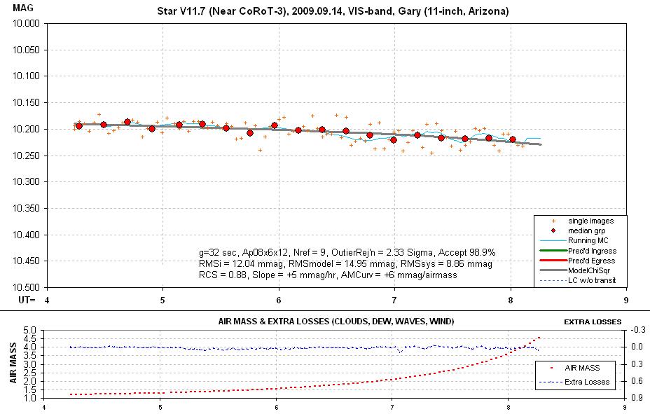
Figure H08. V-band light curve for the V = 10.2 star.

It’s apparent from visual inspection that the i’-band light curve is a better quality one than the V-band light curve. This is also borne out by the quantitative measurements, shown in Fig. A09.

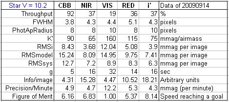
Figure H09. Summary of observations of a star with V = 10.2, brighter than a typical BTE star.

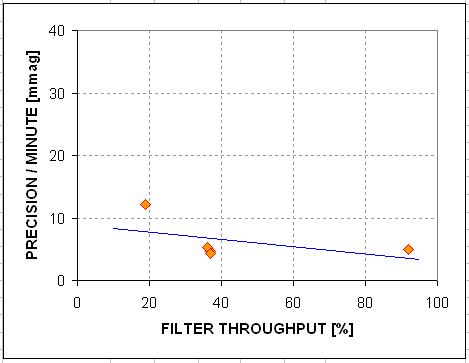
Figure H11. Precision performance versus filter throughput for the V = 10.2 star.

For stars near the bright end of those in the BTE list the best filter for light curves is the i’-band filter. It is 8 times faster than the V-band filter in achieving a specific RMS level of precision. The NIR filter is almost as good, and the CBB and RED filters are close behind.

Concluding Remarks

The results reported here suggest that the best overall filter choice for exoplanet light curve observing is the CBB filter. Brighter exoplanet stars might be observed with greater precision using an i’-band filter, or maybe the NIR filter. For stars ranging in brightness from brighter than typical to the faintest, the worst-performing filter was found to be V-band.

Most of the superior performance of the CBB filter can be attributed to its large throughput. That being the case, why not use a clear filter? As explained in my book Exoplanet Observing for Amateurs (Chapter 14, pages 83 and 84), a clear filter should be avoided for exoplanet light curve observations because it has different effective atmospheric extinction values for red and blue stars (0.132 and 0.191 mmag/airmass), whereas with a CBB filter the two extinction coefficients are almost the same (0.116 and 0.124 mmag/airmass). In other words, the extinction difference between red and blue stars is 59 mmag/airmass for a clear filter and only 8 mmag/airmass for a CBB filter. That’s a 7-fold improvement, which means there should be a 7-fold reduction in the size of the “air mass curvature” systematic error component when using a CBB filter instead of a clear filter. For a typical star the CBB filter passes ~92% of the light passed by the clear filter. This 8% loss is a small penalty for a 7-fold reduction in the “air mass curvature” component of systematic error.

Suppose the amateur community of exoplanet observers started to switch from V and Rc filters to CBB? Would science be lost? Let's review a short list of the science that amateur exoplanet light curves might provide. Transit timing variations (TTV), based on mid-transit times for transits by many observers, can be used to search for another exoplanet in a resonant orbit. TTV can also be used to search for evidence of exomoons. Mid-transit times are unaffected by filter choice, so the better precision afforded by the CBB filter means that this science objective would be enhanced, not compromised. Transit length is predicted to vary if near-grazing  transits are produced by an exoplanet with secular changes in inclination. Transit length is also unaffected by filter choice, so CBB should enhance instead of compromise this science objective. Transit depth may also vary with time if a near-grazing exoplanet changes inclination. Since transit depth varies with filter, differently for each exoplanet, any analysis of amateur data would have to use effective wavelength as an independent variable. Mixing B, V, Rc and Ic measurements means this filter dependence would have to be determined carefully. If most measurements were CBB there would be less need for solving for wavelength dependence in searching for depth changes. If for some reason the science needed to know wavelength dependence, then a call could go out for the object of interest to be observed with B and Ic filters (very few B and Ic data are in the AXA). The science that can be served from transit depth investigations might actually be better served if CBB became the "standard" filter for amateur exoplanet observations. Finally, and this gets to the factor that must be the most troubling to observers active in AAVSO projects, if CBB magnitudes can't be reported on a standard scale (e.g., using CCD Transformation Equations), how can transits be pieced together by many observers? The simple answer is "They can't be!" And this means that ~0.06% of transits in a typical year should not be observed with a CBB filter! Where did this number come from? There are ~5300 transits per year that amateurs can observe, and only three of them are so long that more than one observer is required to properly characterize the transit depth, length and mid-transit time. These are the three transits per year by HD 80606, which has a transit length of ~12.6 hours, that occur at 111.4-day intervals. For these events CBB would only be useful in establishing an ingress time, or an egress time, but none of the observing segments could be properly joined to produce one complete, multiple-observer transit. For the other 45 exoplanets it is true that ~ 1/3 of the light curves in the AXA are partial transits, but even data for ingress-only, or egress-only, can be used in TTV analyses because as complete transits accumulate the transit length becomes well-known, allowing the ingress and egress times to be used to estimate mid-transit times (as I have demonstrated with XO-1, where ~1/2 the LCs are partial). Since very few of the transit events in the AXA are for the same event, the opportunities for joining light curve segments from different observers is negligible. The case for needing to combine observing segments from multiple observers may exist for AAVSO variable stars, but exoplanets are not variable stars.

It is my position that compromises to science from using CBB (or NIR) filters will be not only minimal, but if amateurs switch to CBB and NIR filters the contributions of these observations to science might actually be enhanced because of the improved light curve quality afforded by using these wide bandpass filters. This is a subject worth discussing among the amateur as well as professional community because my views may overlook something important. I welcome feedback on this subject.

To my knowledge this is the first report of results from an observing session designed specifically to identify optimum filter choices for exoplanet light curve observing. There may be flaws in my procedure, and I am open to comments on an improved observing protocol or an improved image analysis protocol. I welcome others to conduct their own “filter playoff” observations, and share them with the community of amateur exoplanet observers. Until others confirm what I have found it is fair to characterize my results as merely “suggestive.” The suggestion, to be explicit, is that the overall best filter choice is CBB-band.

Addendum

The following filter transmission plot shows how the CBB and NIR filters relate to standard filters.

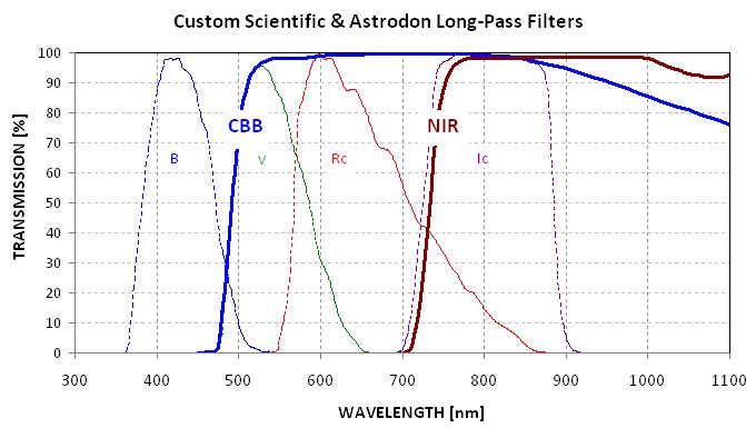
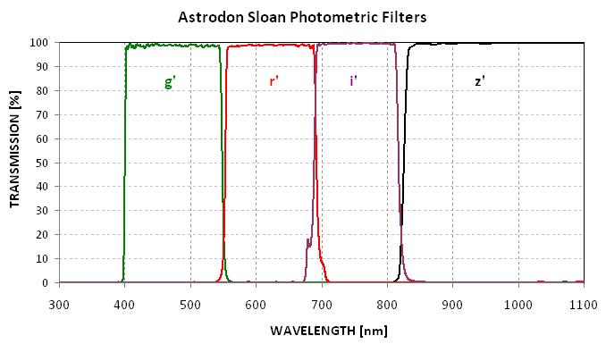
Figure H12. Spectral transmission shapes of the CBB filter (by Custom Scientific), the NIR, B, V, Rc, Ic and SDSS filters g', r', i' and z' (by Astrodon). Transmission functions were kindly provided by Don. S. Goldman, PhD, Astrodon Imaging, Orangevale,CA. 

WebMaster: B. Gary.  This site opened:  2009.09.18, Last Update:  2009.09.20.